Author's posts
Oct 30 2015
Analysing LIDAR data for the UK
I’m currently between jobs for a couple of weeks, so I have time to play with data.
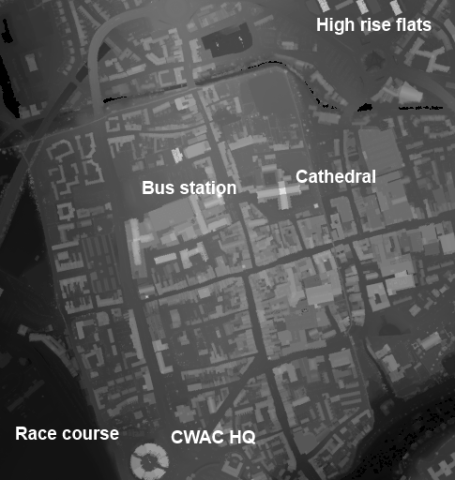
The Environment Agency (EA) has recently released it’s LIDAR data for England amounting to several terabytes of the stuff. LIDAR is a laser ranging technology which gives you the height profile of the surface under inspection. You can get a feel for the data from this excerpt of central Chester:
The brightness of a pixel shows the height of a feature, so the race course (lower left) appears dark since it is a low flat region close to the River Dee. The CWAC HQ building is tall and appears bright. To the north of the city are a set of three high rise flats, which appear bright. The distinctive cross-shape of the cathedral, with it’s high, bright central tower is also visible. It’s immediately obvious that LIDAR is an excellent tool for picking out the footprint of buildings.
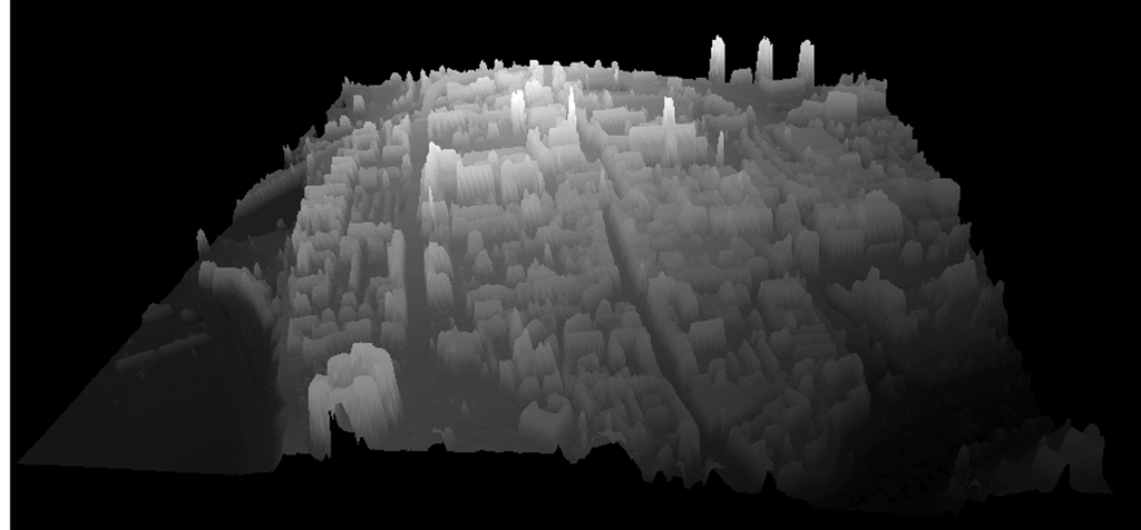
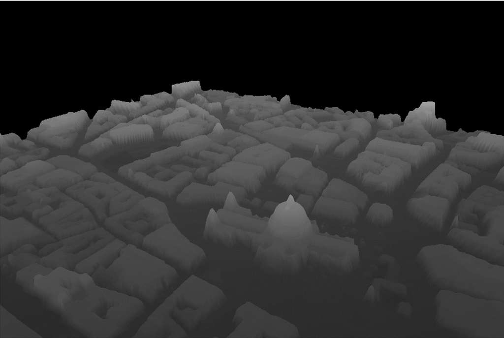
We can use the image above to make a 3D projection view where the brightness of a pixel is mapped to height:
The orientation for this image is the same as that in the first image, the three tower blocks are visible top right, and the CWAC HQ visible lower left.
The images above used the lowest spatial resolution data, each pixel is 2mx2m. The data have released have spatial resolutions 2m down to 25cm for selected areas. Looking at the areas with the high resolution data available it becomes very obvious what the primary uses of the data are: flood and coastal defences.
You can find the LIDAR data here. It’s divided up into several datasets. Surface data gives height information including all objects on the land such as buildings, trees, vehicles and so forth whilst Terrain data is processed to remove these artefacts and show the pristine land surface.
Composite data are data compiled to give maximum coverage by combining data from surveys conducted in different years and at different resolutions whilst Tile data are the underlying raw data collected in different years and different resolutions. The coverage sliders show the coverage of each dataset. The data are for England only.
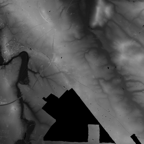
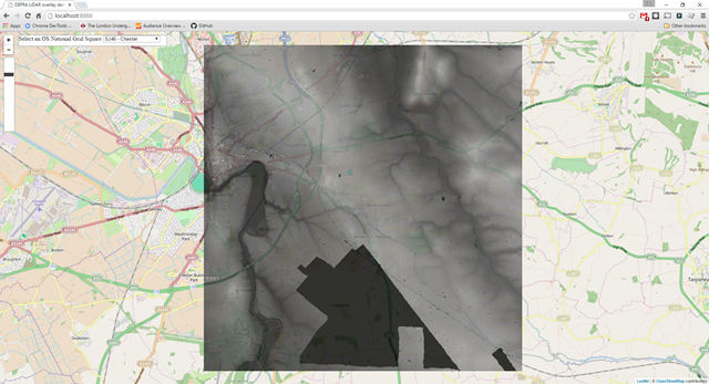
The images of Chester shown above are an excerpt from a 10kmx10km tile, shown below:
Chester is on the left of this image, above the dark bend of River Dee flood plain. To the right hand side we can see the valley of the River Gowy, and its tributaries – features which are not obvious on the ground or in Google Maps. The large black area is where there is no data, smaller irregular black seem to correlate with water, you might just be able to pick out the line of the Shropshire Union canal cutting through the middle of the image.
I used Chester as an illustration because that’s where I live. I started looking at this data because I was curious, and I’ve spent a happy few days downloading data for lots of different places and playing with it.
It’s great to see data like this being released under permissive conditions. The Environment Agency has been collecting this data for its own purposes, and it’s been available from them commercially for a while – no doubt as a result of a central government edict to maximise revenue from it.
Opening the data like this means the curious can have a rummage, and perhaps others will find a commercial value in it.
I’ve included a few more images below. After them you can see the technical details of how to process these data and make the visualisations for yourself, the code is all in this GitHub repository:
https://github.com/IanHopkinson/defra-lidar-viewer
It is shared under the MIT license.
Liverpool in 3D with the Radio City tower
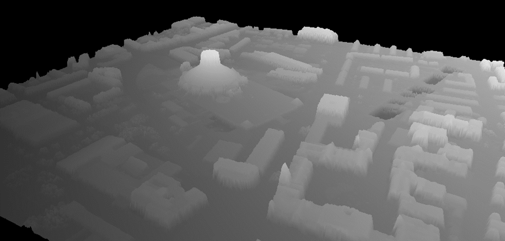
Liverpool Metropolitan Cathedral at 1m resolution
St Paul’s Cathedral
Technical Details
The code used to make the figures in this blog post can be found here:
https://github.com/IanHopkinson/defra-lidar-viewer
The GitHub repository contains a readme file which describes the code, and provides links to the original data, other useful commentary and the numerous bits of code I borrowed from the internet.
The data start as sets of zipped text file archives, each archive contains the data for a 10kmx10km OS National Grid square – Chester is in the SJ46 cell. An archive contains a maximum of 100 text files, each one containing data for a single 1kmx1km square, the size of this file depends on the resolution of the data. I wrote a Python program to read the data for a 10kmx10km cell and convert it into a PNG format image. This program also calculates the bounding box in latitude and longitude for the cell. The processing program works fine for 2m and 1m resolution data. It works just about for 50cm data but is slow and throws memory errors. For 25cm resolution data it doesn’t yet work.
I made a visualisation using the leaflet.js library which allows you to overlay the PNG images generated above onto OpenStreetMap maps. The opacity of the image can be varied with a slider so that you can match LIDAR features to map features. The registration between the two data sources is pretty good but there are systematic problems which I believe might be due to different mapping projections being used by the Ordnance Survey and OpenStreetMap.
A second visualisation tool uses the three.js library to make an interactive 3D view. The input data are manual crops of approximately 512×512 from the raw PNGs, I did this using Paint .NET but other image editors would work fine. Larger images work but they are smoothed to 512×512 in the rendering. A gotcha here is that the revision number of the three.js library is important – the code for this visualisation leant heavily on previous work by others, and whilst integrating new functionality it was important to use three.js source files from the same revision. This visualisation allows you to manipulate the view with the mouse, it takes while to load up but once loaded it is pretty fast. Trying to upload a subsequent image doesn’t work.
I’m still working on the code, I’d like to be able to process the 25cm data and it would be good to select an area from the map and convert it to 3D view automatically.
Oct 20 2015
Book review: High Performance Python by Micha Gorelick & Ian Ozsvald
 High Performance Python by Micha Gorelick and Ian Ozsvald is nominally a book about improving the speed and memory performance of your programs. Along the way it provides insight into some more advanced aspects of Python programming, including how the language works under the hood.
The book starts with tools for analysing the speed and memory performance of programs at global, function and line level. The authors emphasis the importance making these measurements, and using unit testing to ease the process of optimisation. Blindly optimising where you *think* the problem lies is never a good idea.
The next set of chapters talk about some core Python data structures a little about their implementation and relative performance. These include lists and tuples, dictionaries and sets, iterators and generators and matrices and vectors.It is here that the numpy library is introduced, and it is treated almost as a core Python library in its importance.
The difference between range and xrange in Python 2 is striking: if you wish to execute a loop some number of times then range builds a list of size that number of elements and xrange makes a generator and therefore xrange uses far less memory.
The next few chapters cover compiling Python to C for speed increases, concurrency, the multiprocessing module and clusters. Typically chapters take an example (Julia sets, diffusion equations, estimating pi, finding primes) and demonstrate the speedups which can be made, from the routine to the ridiculous. The authors point out when further optimisation is a bit pointless.
For compiling to C, there are a number of options of varying coverage and maturity. Cython offers the most mature, widest coverage but at the cost of making breaking changes to code. Other newer solutions include Numba and PyPy, they do not require breaking changes to code but they are less mature and in the case of PyPy do not support the important numpy library.
Concurrency is about making better use of a single processor using asynchronous methods, here there are libraries such as gevent and tornado.
For parallel processing most focus is on the multiprocessing library, most of the book is platform agnostic but this chapter is based on the Linux implementation of Python.I hadn’t realised before that “embarrassingly parallel” had a specific meaning i.e. that there is no need for interprocess communication for the problem at hand.
The coverage of computing clusters is fairly cursory, this isn’t really the focus of this book and as the authors highlight: running clusters of machines can bring a significant administration overhead.
The book finishes with a chapter on reducing RAM usage, either by choice of intrinsic data types or using probabilistic data structures such as the Bloom filter which offer an approximate answer for vastly less memory usage. Also included are the Morris Counter which provides an approximate counter in 1 byte of storage, I must admit to being bemused as to when I would need such a thing.
Finally, there are what I refer to as “war stories” from practitioners in the field. I really liked these, one of the difficulties in working in technology is the constant stream of options to choose from, often with no clear frontrunner, so learning how others have approached problems is really handy. Here Celery, the Distributed Task Queue, and ElasticSearch get multiple mentions.
Overall the book is well-produced and readable. It occasionally lapses into the problem of inviting the reader to admire the colour in a greyscale printed plot. In other places I felt the example code could have presented up front in its entirety rather than being dribbled out in bits. In the chapter on Using less RAM, I felt important things were discussed (tries and directed-acyclic word graphs (DAWGs) before they were introduced which was a bit confusing. Tries and DAWGs are systems for the compact storage of text, and are both tree-like structures – I hadn’t come across these before.
In some ways this book is more about productionisation rather than performance. For the straightforward non-production data analysis work I’ve done I can imagine being a bit smarter about my choice of data structures and using profiling to be aware the slow points are as a result of this book. In the repeated reanalysis cycle it is nice to have something run in a minute rather than 20, but is it worth a day of development time? I would likely only turn to compilation, concurrency and multiprocessing if I were going to use a particular analysis regularly, or my anticipated run time was going to be measured in days without optimization.
I recommend this book to anyone looking to advance their understanding of Python, and speed up their code.
Oct 10 2015
A Docker environment for Windows (October 2015 edition)
This blog post provides an outline method for installing a nice environment for developing in Python using Docker on a Windows 10 machine. Hopefully I have provided sufficient of the error messages I encountered that both myself and others will find this post when in distress!
The past three years I’ve been working for ScraperWiki as a data scientist, this has meant a degree of coding in Python and interacting with my colleagues, and some customers, who use Linux (principally Ubuntu) or OS X. I have continued to use a Windows laptop. You can see my review of it here.
Until recently my setup was based on a core installation of Python and a whole bunch of handy libraries using Python(x,y). I also installed Git for Windows which gave me a shell prompt, and the command-line git commands along with some fraction of the bash environment. I also installed msysgit which provided further Linux style enhancements to my shell. I configured my shell so I could get ssh access to ScraperWiki servers in the cloud. For reasons I can’t recall I also installed ansicon.exe which gives the Windows Command prompt some of the colour highlighting of a modern shell prompt.
With this setup I could do most of what I needed from Windows, and if I had to I could fire up my Ubuntu VM and work in there. Typically I did this when I had some tricky libraries to install, or I wanted to be sure I could deploy onto ScraperWiki’s servers in the cloud. I never really got virtual environments working nicely on Windows – virtualenvwrapper, which makes such things, nicer is challenging to configure on Windows.
Students of this sort of thing will appreciate that the configuration described above is reached with a degree of trial and error, and a lot of Googling of error messages.
Times have changed and this setup was getting a bit long in the tooth, the environment around me was also changing – we started using Docker. I couldn’t get code using the Python requests library to run because of problems with SSL. Also, all the cool kids were talking about Python 3 and how new projects should all be in Python 3. I couldn’t work out how to add Python 3 to my Python(x,y) installation, and furthermore I was currently tied to 32-bit rather than 64-bit Python. ScraperWiki had recently done some work on making an easily deployable Python application and identified that the Anaconda Python distribution by ContinuumIO was the way to go.
Installing Python 3 and 2 using Anaconda
This worked very smoothly, there is an installer here. I had Python 3.4.3 (64-bit) working in the twinkling of an eye, and from my bash prompt I could now run that Python code which was previously broken due to OpenSSL problems. However, all was not rosy since it turns out my latest project was accidently Python 3 compatible, whilst my older projects were not. I therefore needed Python 2 as well. In principle, with Anaconda this is as simple as doing:
conda create -n python2 python=2.7 anacondaand then
source activate python2This puts you into a Python 2 virtual environment which will run your old code. However, it doesn’t work from the Git Bash prompt, you need to use a Windows Command prompt, as discussed here. But at least I now have the latest whizzy Python 3 installation and I can also run Python 2, when required. It’s worth noting that installing new libraries on Python under Windows has become rather easier with newer versions of pip, I believe due to the introduction of pip wheel. In the past installing some libraries was a pain because of a need to compile binary components.
Using Docker on Windows with Docker Toolbox and the Git SDK
The next task was to get support for Docker, the container system. You can find out more about Docker in my blog post here. Essentially it is a method for running an application in an isolation unit which is defined by a simple Dockerfile, largely removing problems of dependencies and versions. Docker is intrinsically a Linux technology, it relies on several deeply embedded components of the operating system and so does not run on Windows. However, you can boot up a very lightweight Linux-based VM and run Docker images on that from either Windows or OS X. Until recently this was done using boot2docker. The new way is to use the Docker Toolbox. I held off installing this until it became Windows 10 compatible since as a neophile I have obviously upgraded to Windows 10 at earliest opportunity. Docker Toolbox installs VirtualBox to run a VM to host Docker and Git for Windows to provide a bash shell prompt, as well as the Docker commandline tools.
I found installing Docker Toolbox relatively smooth although I had a problem with it finding ssh key files with an error message “open <filepath\ca.pem : The system cannot find the file specified” which was fixed by regenerating the key files:
docker-machine regenerate-certs default
But this alone does not give me the right workflow since ScraperWiki make heavy use of Make to build and run containers and Git for Windows does not come configured with Make. You can see this in action for the Simple API we made for the NewsReader Project. I used the Git for Windows SDK to provide Make and other build tools. This is designed for use by Git for Windows developers, it’s based on msys2 which I also tried to install but which errored on a couple of steps. The Git SDK is more verbose in its installation appeared to install cleanly.
Once we have Git for Windows SDK we need to use its git-bash to launch Docker Quickstart Terminal (rather than the version provided by the Toolbox), this means changing the command executed by the Docker Quickstart Terminal shortcut from:
"C:\Program Files\Git\git-bash.exe" "C:\Program Files\Docker Toolbox\start.sh"
to
C:\git-sdk-64\git-bash.exe "C:\Program Files\Docker Toolbox\start.sh"
Update 2016-03-21: I modified start.sh to give the docker-machine binary an absolute path, this means I can launch a plain Git Bash shell and run the start.sh script later, if required. This change requires further modification to make sure paths were properly escaped. You can see my version of start.sh here: https://gist.github.com/IanHopkinson/85453a90212eb6627f29
Simply trying to run the Git SDK version of the make tool does not seem to work, you get an error like “unable to make temporary trusted Dockerfile”.
We’re into the final straight now!
My final problem was that when I tried to make my previously working application it failed with an error message:
IOError: [Errno 2] No usable temporary directory found in ['/tmp', '/var/tmp', '/usr/tmp', '/home/newsreader-demo']
The problem seems to be the way in which msys2 handles paths in Windows it needs to have two preceding //, rather than one, as described here. So all I need to do is change this line in my Makefile
@docker run -p 8000:8000 --read-only --rm --volume /tmp -e NEWSREADER_PUBLIC_API_KEY ianhopkinson/newsreader_demo
To this:
@docker run -p 8000:8000 --read-only --rm --volume //tmp -e NEWSREADER_PUBLIC_API_KEY ianhopkinson/newsreader_demo
Can you see what I did there?
Update 2015-10-14 – interactive shells into docker
If you try to get an interactive shell on a container then you get an error like:
cannot enable tty mode on non tty input
To avoid this you can use winpty:
winpty docker exec -i -t [CONTAINER_NAME] bash
There’s some discussion of this on the Docker Toolbox issue tracker
Update 2015-10-22 – Which Python are you using?
It turns out I was accidentally using the Python shipped with Git for Windows SDK, rather than the Anaconda version I had so carefully installed. I fixed this by adding this to my .profile file:
export PATH=/c/anaconda3/:$PATH
I didn’t spot it earlier because I checked Python version by running ipython rather than python.
Concluding thoughts
I wrote this partly in frustration at the amount of time I spent getting this all fixed up, and the fact that I couldn’t stop until I had fixed it. The scheme above worked for me but I suspect it is quicker and easier to do on a laptop with no history.
There’s no doubt that the situation is better than I found it 3 years ago but it is still a painful process involving much trial and error. Docker brings great benefits for developers, and once it is working makes sharing your work across multiple users very straightforward.
Sep 30 2015
Book review: The Son also Rises by Gregory Clark
 The Son also Rises by Gregory Clark is a book about social mobility, as traced through surnames. Clark prefaces his work by saying that what he is to say might be considered radical and controversial. Other studies of social mobility have find modest “inheritability” between generations. This study finds high levels of inheritability spanning hundreds of years.
The theme for the early chapters is to find some source of high status individuals – be it graduation from prestigious universities such as Oxford, Cambridge or the American Ivy League, membership of professional bodies such as those for doctors or attorneys or from financial records such as occasional tax releases or records of wills (probate). Next a cohort of names is tracked through these systems and their level of incidence is compared against the background level of incidence for that surname. For example, “Smythe” is a relatively rare surname in the general UK population but it is found at a much higher level in records of registered doctors.
The selected cohort of surnames may be from a distinctive ethnic population – i.e. Japanese in America, Native Americans or French settlers. Or it may be selected from a set of high status individuals at a point in time i.e. the Normans who came the England with William the Conqueror, or Swedish nobles.
Clark’s discovery is that for all of these many cohorts across multiple measures of status the persistence over time is strong. The Smythes of 200 years ago had relatively high status then and they still do now. After nearly a 1000 years those with surnames associated with the Norman conquest are still a little over-represented in the intake of Oxford and Cambridge University. Similar behaviour is found for low status groups, Baldrick’s character through the several series of Blackadder is not far from the truth. In both cases these groups are “regressing towards the mean” but it is a long, slow process.
Following these initial demonstrations of social mobility, Clark states his general law which is that the correlation of status over generations is high compared to previously measured parent-child measures and remarkably constant across multiple countries, periods in history and cohorts. The magic number for the correlation is 0.75. He argues that the reason that his estimate is higher than others is that he models social mobility with an underlying constant and a random fluctuation, the methods of calculation for early figures mean that this random fluctuation is much more apparent and brings down the measured social mobility. I don’t feel he demonstrates the origin of this discrepancy very clearly.
Subsequent chapters go on to look at some cases where one really expects deviations from this general rule, in the Indian caste system where low mobility is expected and also in China, where post-revolution is expected to be a time of high social mobility. It turns out that in India, despite laws aimed at reducing caste based discrimination, social mobility is has not improved dramatically. In China social mobility seems to have been little bothered by the revolution. The odd groups that do break the rule of constant social mobility seem to do so by preferential recruitment i.e. in the past in Muslim countries non-Muslims were tolerated but charged a poll tax which meant that lower status/income people were more likely to convert to Islam leaving a more persistently high status non-Muslim population. A second route is by strong preference for “in group” marriage which is seen in the Indian Brahmin caste. It turns out that the surnames identified with British parliamentarians are particularly immobile.
As for the origin of this constant social mobility, Clark ascribes it to what he calls “social competence”. There is a confused discussion of the balance of nature and nurture, not helped by a table where nature and nurture headings are accidently swapped (I think). I believe that technically it is all nurture, and Clark is trying to work out whether it is all about money. It strikes me that your wider family is where you learn about what the possibilities are for you and, while every family has it’s black sheep, the fact that your father, two out of three uncles went to Cambridge University means that your expectation is that you should aspire to that. Your family sets what is “normal”.
I suspect that this is particularly the case for British parliamentarians where there seems to be a lot of siblings (Milibands, Johnsons, Eagles), husband wife (Cooper/Balls) and parent-child (Kinnock, Benn) combinations. Being a politician is an odd sort of job, there is not really a class at school for it, seeing your family working in the “family business” must be a big influence.
“The Son also Rises” is an interesting read but turning it into a 300 page book seems to belabour the point somewhat. I liked the incidental details of the origins of surnames, and the various sources of information on social status.
I got this as a Kindle edition, I wish I’d bought it as a paperback, there are numerous figures, tables and equations which didn’t render at a reasonable size in the first instance.
Sep 21 2015
Book review: The Values of Precision edited by M. Norton Wise
 The Values of Precision edited by M. Norton Wise is a collection of essays from the Princeton Workshop in the History of Science held in the early 1990s.
The essays cover the period from the mid-18th century to the early 20th century. The early action is in France and moves to Germany, England and the US as time progresses. The topics vary widely, starting with population censuses, then moving on to measurement standards both linear and electrical, calculating methods and error analysis.
I’ve written some notes on each essay, skip to the end of the bullet points if you want the overview:
- The first article is about the measurement of population, mainly in pre-revolutionary France. This was spurred by two motivations: firstly, monarchs were increasingly seeing the number of their subjects as a measure of their power and secondly, there was a concern that France was experiencing depopulation. In the 17th century the systematic recording of births, deaths and marriages was mandated by royal direction. In the period after this populations were either estimated from a count of “hearths” or from the number of births. The idea being that you could take either of these indirect measures and multiple them by some factor to get a true measure of population.
- The second article is by Ken Alder, he of “The Measure of All Things” and is another trip to revolutionary France and their efforts to introduce a metric system of measurement. The revolutionary attempt failed but the system of standards they created prevailed in the middle of the 19th century but not without some effort. Alder highlights the resistance of France to metrification, and also how the revolution bred a will to introduce a rational system based on natural measurements rather than a physical object created by man. He also discusses some of the benefits of the pre-metric system: local control, the ability for workers to take a cut without varying price, connection to effort expended/quality. This last because land was measured in terms of the amount of grain used to seed it or the area one person could harvest in a day – this varies with the quality of the land.
- Jan Golinski writes on Lavoisier (again from France at the turn of the Revolution) regarding “exactness” and its almost political nature. Lavoisier made much of his exact measurements in the determination of the masses of what are now called hydrogen and oxygen in producing a known mass of water. This caused some controversy since other experimenters of the time saw his claims of exactness in measurement to be mis-used in supporting his theory for chemical reactions. There were reasons to be sceptical of some of his claims, he often cited weighed amounts to more significant figures than were justified by the precision of his measurements and there are signs his recorded measurements are a little too good to be true. These could be seen as the birthing pains of a new way of doing science which didn’t just apply to chemical measurements of the time, but also to surveying and the measurement of population. These days the inappropriateness quoting of more significant figures than are justified by the measurement is drummed into students at an early age.
- Next we move from France to Germany and a discussion of the method of least squares, and the authority of measurements by Kathryn M. Olesko. Characters such as Legrendre and Laplace had started to put the formal analysis of error and uncertainty in measurement on the map. This work was carried forward by Gauss with the method of least squares, essentially this says that the “true” value of a measurement is that which minimises the squared difference of all the measurements made of that value. It is an idea related to probability, and it is still deeply embedded in how we make measurements today and also how we compare measurement to theory. In common with events in France, the drive for better measurement came in Germany with a drive to standardise weights and measures for the purposes of trade. The action here takes place in the first half of the 19th century.
- The trek through the 19th century continues with Simon Schaffer’s essay on the work in England and Germany on electrical units with a particular view to establishing whether the speed of light and the speed of propagation of electromagnetic waves were the same. This involved the standardisation of units of electrical resistance. It was work that went on for some time. Interesting from a practicing scientists point of view was the need for the bench scientist and instrument makers to work closely together.
- The next chapter is a step away from the physical sciences with a look at life insurance and the actuarial profession in the first half of the 19th century. Theodore Porter describes the attitude of this industry to precision and calculation, noting that they fended off attempts to regulate the industry too tightly by arguing that there business could not be reduced to blind calculation. The skill, judgement and character of the actuary was important.
- The Image of Precision is about Helmholtz’s work on muscle physiology in around 1850, he used an apparatus which showed the extension of a muscle graphically following stimulation, and measured the speed of nerve impulses using similar methods. The graphical method was in some senses less precise than an alternative method but it was a more compelling explanatory tool and provided for better understanding of the phenomena under study.
- Next up is a discussion of the introduction of so-called “direct-reading” ammeters and voltmeters by Ayrton and Perry in around ~1870. This was an area of some dispute, with physicists claiming that determinations of volts and amps be made by reference to the basic units of length, time and mass. Ayrton and Perry were interested in training electrical engineers whose measurements would be made in environments not conducive to these physicist-preferred measurements. Not conducive in both a technical sense (stray magnetic fields, vibration and so forth) nor in the practical sense (an answer within 1 percent in 10 minutes was far superior to one within 0.5 percent in 2 hours).
- As we approach the end of the book we learn of Henry Rowland, and his diffraction gratings, made at John Hopkins university. Rowland had toured Europe, and on his return set to making high quality diffraction gratings to measure optical spectra. This is a challenging technical task, to be useful a diffraction grating needs many very closely spaced lines of the same profile. Rowland sent out his diffraction gratings for a nominal price, making no profit, but did not reveal the details of his methods. It took many years for his work to be better, and even longer yet for better diffraction gratings to be available generally.
- The collection finishes with the construction of mathematical tables, starting with a somewhat philosophical discussion of the limits of calculation but moving onto more pragmatic issues of the calculation and sharing tables. The need for these tables came original with the computationally intensive calculations for determining the longitude by the method of lunar distances. The 19th century saw the growth in mathematical analysis in a range of areas, spreading the need to make mathematical tables. Towards the end of the century machine calculation was used to help build these tables, and do the analysis they supported. Students of my generation will likely just about remember using tables of trigonometric and other functions, these days in my practical work they are entirely replaced by computer calculations done on demand.
There is a lot in here which will speak to those with a training in science, physics in particular. The techniques discussed and the concerns of the day we will recognise in our own training. The essays hold a slight distance from practitioners in this arts but that brings the benefit of a different view. Core to which is the way in which precision in measurement is a social as well as technical affair. To propagate standards of measurement requires the community to build trust in the work of others, this does not happen automatically.
I like this style of presentation, each essay has its own character and interest. The range covered is much larger than one might find in a book length biography, and there is a degree of urgency in the authors getting their key points across in the space allocated.
In this book the various chapters do not overlap in their topics and cover a substantial period in time and space with the editor providing some short linking chapters to tie things together. All in all very well done.

