Tag: SQL

Book review: Essential SQLAlchemy by Jason Myers and Rick Copeland

sqlalchemyEssential SQLAlchemy by Jason Myers and Rick Copeland is a short book about the Python library SQLAlchemy which provides a programming interface to databases using the SQL query language. As with any software library there is ample online material on SQLAlchemy but I’m old-fashioned and like to buy a book.

SQL was one of those (many) things I was never taught as a scientific programmer, so I went off and read a book and blogged about it (rather more extensively than usual). It’s been a useful skill as I’ve moved away from the physical sciences to more data-oriented software development. As it stands I have a good theoretical knowledge of SQL and databases, and can write fairly sophisticated single table queries but my methodology for multi-table operations is stochastic.

I’m looking at using SQLAlchemy because it’s something I feel I should use, and people with far more experience than me recommend using it, or a similar system. Django, the web application framework, has its own ORM.

Essential SQLAlchemy is divided into three sections, on SQLAlchemy Core, SQL Alchemy ORM and Alembic. The first two represent the two main ways SQLAlchemy interacts with databases. The Core model is very much a way of writing SQL queries but with Pythonic syntax. I can see this having pros and cons. On the plus side I’ve seen SQLAlchemy used to write, succinctly, rather complex join queries. In addition, SQLAlchemy Core allows you to build queries conditionally which is possible by using string manipulation on standard queries but requires some careful thought which SQLAlchemy has done for you. SQLAlchemy allows you to abstract away the underlying database so that, in principle, you can switch from SQLite to PostgresQL seamlessly. In practice this is likely to be a bit fraught since different databases support different functionality. This becomes a problem when it becomes a problem. SQLAlchemy gives your Python programme a context for its queries which I can see being invaluable in checking queries for correctness and documenting the database the programme accesses. On the con side: I usually know what SQL query I want to write, so I don’t see great benefit in adding a layer of Python to write that query.

SQLAlchemy Object Relational Mapper (ORM)  is a different way of doing things. Rather than explicitly writing SQL-like statements we are invited to create classes which map to the database via SQLAlchemy. This leaves us to think about what we want our classes to do rather than worry too much about the database. This sounds fine in principle but I suspect the experienced SQL-user will know exactly what database schema they want to create.

Both the Core and ORM models allow the use of “reflection” to build the Pythonic structures from a pre-existing datatabase.

The third part of the book is on Alembic, a migrations manager for SQLAlchemy, which is installed separately. This automates the process of upgrading your database to a new schema (or downgrading it). You’d want to do this to preserve customer data in a transactional database storing orders or something like that. Here I learnt that SQLite does not have full ALTER TABLE functionality.

A useful pattern in both this book and in Test-driven Development is to wrap database calls in their own helper functions. This helps in testing but it also means that if you need to switch database backend or the library you are using for access then the impact is relatively low. I’ve gone some way to doing this in my own coding.

The sections on Core and ORM are almost word for word repeats with only small variations to account for the different syntax between the two methods. Although it may have a didactic value this is frustrating in a book already so short.

Reading this book has made me realise that the use I put SQL to is a little unusual. I typically use a database to provide convenient access to a dataset I’m interested in, so I do a one off upload of the data, apply indexes and then query. Once loaded the data doesn’t change. The datasets tend to be single tables with limited numbers of lookups which I typically store outside of the database. Updates or transactions are rare, and if I want a new schema then I typically restart from scratch. SQLite is very good for this application. SQLAlchemy, I think, comes into its own in more transactional, multi-table databases where Alembic is used to manage migrations.

Ultimately, I suspect SQLAlchemy does not make for a whole book by itself, hence the briefness of this one despite much repeated material. Perhaps, “SQL for Python Programmers” would work better, covering SQL in general and SQLAlchemy as a special case.

Inordinately fond of bottles…

J.B.S. Haldane, when asked “What has the study of biology taught you about the Creator, Dr. Haldane?”, he replied:
“I’m not sure, but He seems to be inordinately fond of beetles.”

The National Museum of Science & Industry (NMSI) has recently released a catalogue of its collection in easily readable form, you can get it here. The data includes descriptions, types of object, date made, materials, sizes, and place made – although not all objects have data for all these items. Their intention was to give people an opportunity to use the data, now who would do such a thing?

The data comes in four 16mb CSV files plus a couple of other smaller ones covering the media library (pictures) and a small “events” library. I’ve focussed on the main catalogue. You can load these files individually into Microsoft Excel, each one has about 65536 rows so they’re a bit of a pain to use, alternatively you can upload them to a SQL database. This turns out to be exceedingly whizzy! I wrote a few blog posts about SQL a while back as I learnt about it and this is my first serious attempt to use it. Essentially SQL allows you to ask nearly human language looking questions of big datasets, like this:

USE sciencemuseum;
SELECT collection,
COUNT(collection)
FROM   sciencemuseum.objects
GROUP  BY collection
ORDER  BY COUNT(collection) DESC
LIMIT  0, 11000; 

This gets you a list of all the collections inside the Science Museums catalogue (there are 162) and tells you how many objects are in each of these collections. Collections have names like “SRM – Acoustics” and “NRM – Railway Timepieces”, the NMSI incorporates the National Railway Museum (NRM), and the National Media Museum (NMEM) as well as the Science Museum (SCM) – hence the first three letters of the collection name. I took the collection data and fed it into Many Eyes to make a bubble chart:
The size of the bubble shows you how many objects are in a particular collection, you can see a majority of the major collections are medical related. So what’s in these collections? As well as longer descriptions, many objects are classified into a more limited number of types. This bubble chart shows the number of objects of each type:

This is where we learn that the Science Museum is inordinately fond of bottles (or jars, or specimen jars, or albarello’s or “shop rounds”). There are also a lot of prints and posters, from the National Railway Museum. This highlights a limitation to this type of approach: the fact that there are many of an object tells you little. It perhaps tells you how pervasive medicine has been in science – it is the visible face of science and has been for many years.

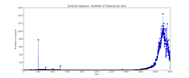
I have also plotted when the objects in the collection were made:

This turns out to be slightly tricky since over the years different curators have had different ideas about how *exactly* to describe the date when an object was made. Unsurprisingly in the 19th century they probably didn’t consider that a computer would be able to process 200,000 records in 1/4 second but simultaneously be unable to understand that circa 1680, c. 1680, c1680, ca 1680 and ca. 1680 actually all mean the same thing. This shows a number of objects in the first few centuries AD, followed by a long break and gradual rise after 1600 – the period of the Scientific Revolution. The pace picks up once again at the beginning of the 19th century.

I also made a crack at plotting where all the objects originating in the UK came from, on PC this is a live Google Map and is zoomable, beneath the red bubbles are disks sized in proportion to the number of objects from that location:

From this I learnt that there was a Pilkingtons factory in St Asaph, and a man in Chirk made railway models. To me this is the value of programming, the compilers of the catalogue made decisions as to what they included but once in my hands I can look into the catalogue according to my interests. I can explore in my own way, if I were a better programmer I could perhaps present you with a slick interface to do the same.

Finally for this post, I tried to plot when the objects arrived at the museum, this was a bit tricky: for about 60% of the objects the object reference number for objects contains the year as the first four characters so I just have the data for these:

The Science Museum started in 1857, the enormous spike in 1889 is due to the acquisition of the collection of Sir John Percy on his death, I discovered this on the the Science Museum website. Actually, I’d like to commend the whole Science Museum site to you, it’s very nice.

I visited the Science Museum a number of times in my childhood, I must admit to preferring it to the Natural History Museum, which seemed to be overwhelming large. The only record I have of these visits is this picture of a German Exchange visit to the museum, in 1985:

I must admit to not being a big fan of museums and galleries, they make my feet ache and I can’t find what I’m looking for or I don’t know what I’m looking for, and there never seems to be enough information on the things I’m looking at. This adventure into the data is my way of visiting a museum, I think I’ll spend a bit more time in wandering around the museum.

I had an alternative title for people who had never heard of J.B.S. Haldane: “It’s full of jars”

Footnote
If the Many Eyes visualisation above don’t work, you can see them in different formats from my profile page.

A set of blog posts on SQL

This is a roundup post for a rather specialist set of posts I wrote on SQL (Structured Query Language), a computer language for creating and querying databases. Basically the posts are my notes on the language which I’m learning because a couple of programming projects I have in mind will need it. The main source for these notes is the Head First SQL book. I’ve used a another book in this series (Head First Design Patterns) – I quite like the presentational style. The code in the posts is formatted for display using this SQL to HTML formatter.

Topics covered:
Some notes on SQL: 1 – Creation
Some notes on SQL: 2 – Basic SELECT
Some notes on SQL: 3 – Changing a table
Some notes on SQL: 4 – Advanced SELECT
Some notes on SQL: 5 – Database design
Some notes on SQL: 6 – Multi-table operations
Some notes on SQL: 7 – Subqueries and views

Of course you can find SQL cheatsheets elsewhere.

The Head First SQL book also has material on transactions and security, if I get a renewed bout of enthusiasm I will add a post on these items.

I used MySQL via its command line client to do the exercises, because it’s about as straightforward as you can get. Notepad++ recognises SQL as a language and will do syntax highlighting, so I type my commands into it and copy them into the MySQL command line client. MySQL is pretty straightforward to install. I also installed Microsoft SQL Server Express 2008, which turned out to be a bit more of a struggle but on the plus side integration the C# .NET, which is what I normally program in, looks better than for MySQL.

I’ve been using with the SQL Server via SQL Management Studio (a graphical interface to databases) on the general election data compiled by The Guardian. First contact with actual data, as opposed to learning exercises has proved interesting! A lot of things that are fiddly to do in a spreadsheet are straightforward using  SQL.

SQL was designed in the early 1970’s, with commercial implementations appearing towards the end of the decade. It’s influence visible is visible in more modern languages, such as the LINQ extensions to C# (this influence is pretty explicitly stated). Some of the ideas of database design (normalisation) seem relevant to object-oriented programming.

It’s been an interesting learning experience, my scientific background in programming has me stuffing pretty much any sort of data into an array in the first instance. SQL and a database look like a much better solution for many situations.

Some notes on SQL: 7 – Subqueries, combining selections and views

This is the seventh, and final, in a series of blog posts on SQL, the first covered creating a database, the second selecting information from a database, the third commands to modify the structure and contents of an existing database, the fourth, advanced selection. The fifth post covered database design. The sixth post covered multi-table database operations. This post covers subqueries and views. No claim of authority is made for these posts, they are mainly intended as my notes on the topic.
This is largely a wrapping up blog post to cover a couple of items.As an alternative to the joins described in a previous post, “subqueries” can often be used. A subquery is essentially an entire query embedded in another query. Subqueries can be used with UPDATE, INSERT and DELETE statements, whilst joins cannot. However, joins can be used to bring columns from multiple tables. There are no special keywords involved in creating a subquery. There is some discussion on the pros and cons of subqueries and joins here on Stackoverflow.

In an uncorrelated subquery the so-called inner query can be evaluated with no knowledge of the contents of the outer query. This expression contains an uncorrelated subquery:

UPDATE raw_candidate_data
SET    gender = ‘f’
WHERE  firstname IN (SELECT firstname
FROM   firstname_gender_lookup
WHERE  gender = ‘f’); 

The inner query is the clause in brackets, in this instance it is a shorthand way of building a list for an “IN” comparison. Often an inner query returns a single value, i.e. for an average or maximum in a list.

This expression contains a correlated subquery:

UPDATE raw_candidate_data
SET    party_id = (SELECT party_id
FROM   parties
WHERE  raw_candidate_data.party = parties.party_name); 

The inner query requires information from the outer query to work, this expression acts as a look up.

Complex queries can be given aliases using the VIEW keyword, for example:

CREATE VIEW web_designer AS SELECT mc.first_name, mc.last_name, mc.phone,
mc.email FROM my_contacts mc NATURAL JOIN job_desired jd WHERE jd.title=‘Web Designer’; 

Can subsequently be used by:

SELECT * FROM   web_designers; 

The view web_designers can be treated just as any other table.

The results of multiple select commands can be combined using the keywords: UNION, UNION ALL, INTERSECT and EXCEPT. UNION returns the distinct union of the results of all the selects, i.e. with no repeats, UNION ALL includes the repeats. INTERSECT returns items that are common to both SELECTs and EXCEPT returns those items that are returned by the first SELECT but not the second. The general form for these combination operations is as follows:

SELECT title FROM   job_current
UNION
SELECT title FROM   job_desired
UNION
SELECT title FROM   job_listings
ORDER  BY title; 

Each SELECT statement must return the same number of columns and each column must be coercible to the same datatype. Only a single ORDER BY statement for the set of SELECTs can be used.

Keywords: UNION, UNION ALL, INTERSECT, EXCEPT, VIEW

Some notes on SQL: 6 – Multi-table operations

This is the sixth in a series of blog posts on SQL, the first covered creating a database, the second selecting information from a database, the third commands to modify the structure and contents of an existing database, the fourth, advanced selection. The fifth post covered database design. This post covers multi-table database operations. No claim of authority is made for these posts, they are mainly intended as my notes on the topic.

Good database design leads us to separate information into separate tables, the information we require from a SELECT statement may reside in multiple tables. There are keywords and methods in SQL to help with extracting data from multiple tables. To assist with clarity aliases, indicated using the AS keyword, allow tables to be given shorter, or clearer, names temporarily. Various JOIN keywords enable lookups between tables, as with other aspects of SQL there are multiple ways of achieving the same results – in this case ‘subqueries’.

The AS keyword can be used to populate a new table with the results of a SELECT statement, or it can be used to alias a table name. In it’s aliasing guise it can be dropped, in shorthand. This is AS being used in table creation:
CREATE TABLE profession
(
id         INT(11) NOT NULL AUTO_INCREMENT PRIMARY KEY,
profession VARCHAR(20)
) AS
SELECT profession
FROM   my_contacts
GROUP  BY profession
ORDER  BY profession;

The following two forms are equivalent, the first uses the AS to alias, the second uses an implicit alias:
SELECT profession AS mc_prof
FROM   my_contacts AS mc
GROUP  BY mc_prof
ORDER  BY mc_prof;


SELECT profession mc_prof
FROM   my_contacts mc
GROUP  BY mc_prof
ORDER  BY mc_prof;


The following examples use two tables boys which is a three column table {boy_id, boy, toy_id} and toys a two column table {toy_id, toy}.

boy_id boy toy_id
1 Davey 3
2 Bobby 5
3 Beaver 2
4 Richie 1
toy_id toy
1 Hula hoop
2 balsa glider
3 Toy soldiers
4 Harmonica
5 Baseball cards

Cross, cartesian, comma join are all names for the same, relatively little used operation which returns every row from one table crossed with every row from a second table, that’s to say two 6 row tables will produce a result with 36 rows. Although see here for an application.
SELECT t.toy,
b.boy
FROM   toys AS t
CROSS JOIN boys AS b;

Notice the use of the period and aliases to reference columns, this query will produce a 20 row table.

Inner join combines the rows from two tables using comparison operators in a condition, an equijoin returns rows which are the same, a non-equijoin returns rows that are different. These are carried out with the same keywords, the condition is different. This is an equijoin:
SELECT boys.boy,
toys.toy
FROM   boys
INNER JOIN toys
ON boys.toy_id = toys.toy_id;

The ON and WHERE keywords can be used interchangeable; in this instance we do not use aliases furthermore since the columns in the two tables (toys and boys) have the same name we could use a natural join:
SELECT boys.boy,
toys.toy
FROM   boys
NATURAL JOIN toys;


Natural join is a straightforward lookup operation, a key from one table is used to extract a matching row from a second table, where the key column has the same name in each table. Both of these versions produce the following table:

boy toy
Richie hula hoop
Beaver balsa glider
Davey toy soldiers
Bobby harmonica


A non-equijoin looks like this:
SELECT boys.boy,
toys.toy
FROM   boys
INNER JOIN toys
ON boys.toy_id<>toys.toy_id
ORDER  BY boys.boy;

the resultant in this instance is four rows for each boy containing the four toys he does not have.

Outer joins are quite similar to inner joins, with the exception that they can return rows when no match is found, inserting a null value. The following query
SELECT b.boy,
t.toy
FROM   boys b
LEFT OUTER JOIN toys t
ON b.toy_id = t.toy_id;

produces this result

Boy toy
Richie Hula hoop
Beaver balsa glider
Davey Toy soldiers
NULL Harmonica
Bobby Baseball cards

That’s to say each row of the toys table is taken and matched to the boys table, where there is no match (for toy_id=4, harmonica) a null value is inserted in the boy column. Both LEFT OUTER JOIN and RIGHT OUTER JOIN are available but the same effect can be achieved by swapping the order in which tables are used in the query.


In some instances a table contains a self-referencing foreign key which is the primary key of the table. An example might be a three column table, clown_info, of “clowns” {id, name, boss_id} where each id refers to a clown name and the bosses identified by boss_id are simply other clowns in the same table. To resolve this type of key a self-join is required this uses two aliases of the same table.
SELECT c1.name,
c2.name AS boss
FROM   clown_info c1
INNER JOIN clown_info c2
ON c1.boss_id = c2.id; 


Notice both c1 and c2 alias to clown_info.

Keywords: AS, ON, INNER JOIN, NATURAL JOIN, LEFT OUTER JOIN, RIGHT OUTER JOIN, UNION, INTERSECT, EXCEPT