I’m currently between jobs for a couple of weeks, so I have time to play with data.

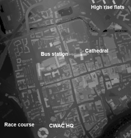
The Environment Agency (EA) has recently released it’s LIDAR data for England amounting to several terabytes of the stuff. LIDAR is a laser ranging technology which gives you the height profile of the surface under inspection. You can get a feel for the data from this excerpt of central Chester:

The brightness of a pixel shows the height of a feature, so the race course (lower left) appears dark since it is a low flat region close to the River Dee. The CWAC HQ building is tall and appears bright. To the north of the city are a set of three high rise flats, which appear bright. The distinctive cross-shape of the cathedral, with it’s high, bright central tower is also visible. It’s immediately obvious that LIDAR is an excellent tool for picking out the footprint of buildings.

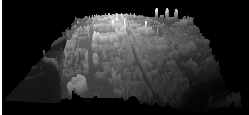
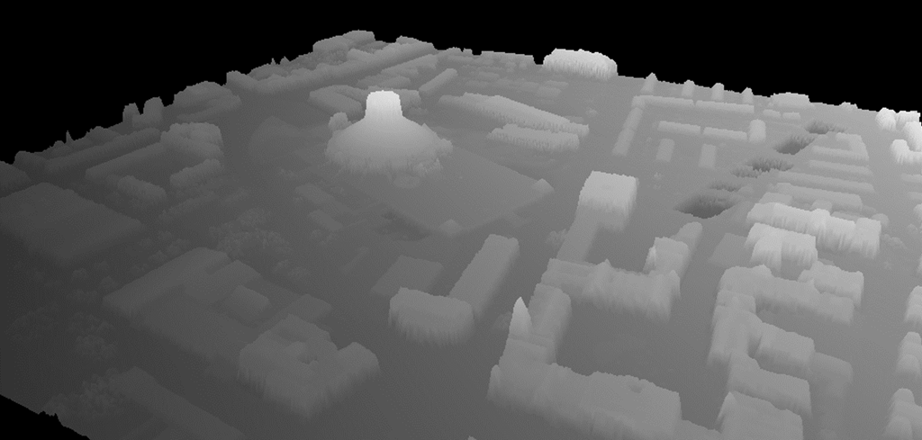
We can use the image above to make a 3D projection view where the brightness of a pixel is mapped to height:

The orientation for this image is the same as that in the first image, the three tower blocks are visible top right, and the CWAC HQ visible lower left.

The images above used the lowest spatial resolution data, each pixel is 2mx2m. The data have released have spatial resolutions 2m down to 25cm for selected areas. Looking at the areas with the high resolution data available it becomes very obvious what the primary uses of the data are: flood and coastal defences.

You can find the LIDAR data here. It’s divided up into several datasets. Surface data gives height information including all objects on the land such as buildings, trees, vehicles and so forth whilst Terrain data is processed to remove these artefacts and show the pristine land surface.

Composite data are data compiled to give maximum coverage by combining data from surveys conducted in different years and at different resolutions whilst Tile data are the underlying raw data collected in different years and different resolutions. The coverage sliders show the coverage of each dataset. The data are for England only.

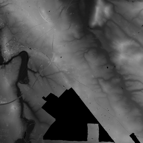
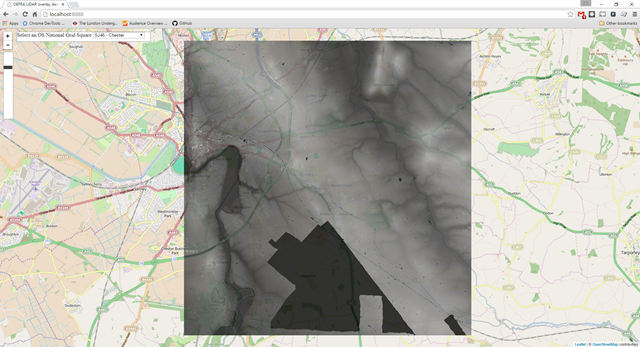
The images of Chester shown above are an excerpt from a 10kmx10km tile, shown below:

Chester is on the left of this image, above the dark bend of River Dee flood plain. To the right hand side we can see the valley of the River Gowy, and its tributaries – features which are not obvious on the ground or in Google Maps. The large black area is where there is no data, smaller irregular black seem to correlate with water, you might just be able to pick out the line of the Shropshire Union canal cutting through the middle of the image.

I used Chester as an illustration because that’s where I live. I started looking at this data because I was curious, and I’ve spent a happy few days downloading data for lots of different places and playing with it.

It’s great to see data like this being released under permissive conditions. The Environment Agency has been collecting this data for its own purposes, and it’s been available from them commercially for a while – no doubt as a result of a central government edict to maximise revenue from it.

Opening the data like this means the curious can have a rummage, and perhaps others will find a commercial value in it.

I’ve included a few more images below. After them you can see the technical details of how to process these data and make the visualisations for yourself, the code is all in this GitHub repository:

https://github.com/IanHopkinson/defra-lidar-viewer

It is shared under the MIT license.

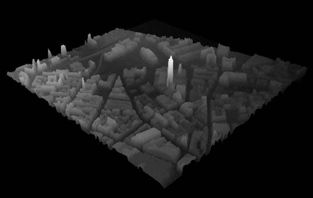
Liverpool in 3D with the Radio City tower

Liverpool Metropolitan Cathedral at 1m resolution

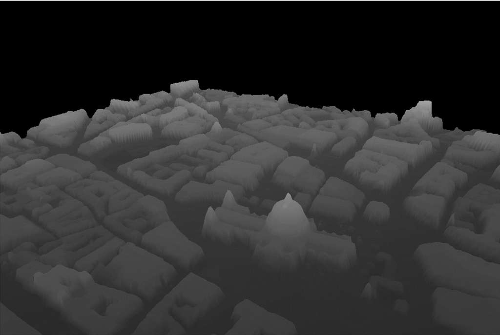
St Paul’s Cathedral

Technical Details

The code used to make the figures in this blog post can be found here:

https://github.com/IanHopkinson/defra-lidar-viewer

The GitHub repository contains a readme file which describes the code, and provides links to the original data, other useful commentary and the numerous bits of code I borrowed from the internet.

The data start as sets of zipped text file archives, each archive contains the data for a 10kmx10km OS National Grid square – Chester is in the SJ46 cell. An archive contains a maximum of 100 text files, each one containing data for a single 1kmx1km square, the size of this file depends on the resolution of the data. I wrote a Python program to read the data for a 10kmx10km cell and convert it into a PNG format image. This program also calculates the bounding box in latitude and longitude for the cell. The processing program works fine for 2m and 1m resolution data. It works just about for 50cm data but is slow and throws memory errors. For 25cm resolution data it doesn’t yet work.

I made a visualisation using the leaflet.js library which allows you to overlay the PNG images generated above onto OpenStreetMap maps. The opacity of the image can be varied with a slider so that you can match LIDAR features to map features. The registration between the two data sources is pretty good but there are systematic problems which I believe might be due to different mapping projections being used by the Ordnance Survey and OpenStreetMap.

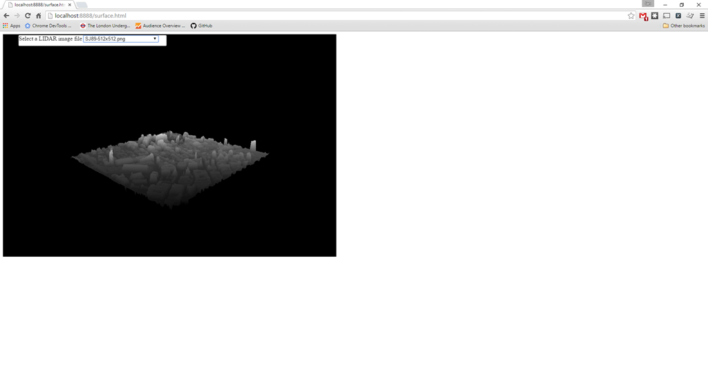
A second visualisation tool uses the three.js library to make an interactive 3D view. The input data are manual crops of approximately 512×512 from the raw PNGs, I did this using Paint .NET but other image editors would work fine. Larger images work but they are smoothed to 512×512 in the rendering. A gotcha here is that the revision number of the three.js library is important – the code for this visualisation leant heavily on previous work by others, and whilst integrating new functionality it was important to use three.js source files from the same revision. This visualisation allows you to manipulate the view with the mouse, it takes while to load up but once loaded it is pretty fast. Trying to upload a subsequent image doesn’t work.

I’m still working on the code, I’d like to be able to process the 25cm data and it would be good to select an area from the map and convert it to 3D view automatically.