Author's posts
Aug 26 2015
Book Review: Stargazers–Copernicus, Galileo, the Telescope and the Church by Allan Chapman
 It’s been a while since my last book review here but I’ve just finished reading Stargazers: Copernicus, Galileo, the Telescope and the Church by Allan Chapman.
The book covers the period from the end of the 16th century, the time of Copernicus and Tycho Brahe, to the early 18th century and Bradley’s measurement of stellar aberration passing Galileo, Newton and others on the way. Conceptually this spans the full transition from a time when people believed in a Classical universe with earth at its centre, and stars and planets plastered onto crystal spheres, to the modern view of the solar system with the earth and other planets orbiting the sun.
This development parallels that in Arthur Koestler’s classic book "The Sleepwalkers”, however Chapman’s style is much more readable, his coverage is broader but not so deep. Chapman introduces a wealth of little personal anecdotes and experiments. For instance on visiting Tycho Brahe’s island observatory he recounts a meeting with a local farmer who had in his living room a marked stone from the Brahe’s observatory (which had been dismantled by the locals on Brahe’s death). Brahe was hated by his tenants for his treatment of them, a hate that was handed down through the generations. Illustrations are provided in the author’s own hand, which is surprisingly effective. He discusses his own work in reconstructing historical apparatus and observations.
Astronomy was an active field from well before the start of this period for a couple of reasons: firstly, astrology had been handed down from Classical times as a way of divining the future. To was believed that to improve the accuracy of astrological predictions better data on the locations of heavenly bodies over time was required. Similarly, the Christian Church required accurate astronomical measurement to determine when Easter fell, across increasingly large spans of the Earth.
The period covered by the book marks a time when new technology made increasingly accurate measurements of the heavens possible, and the telescope revealed features such as mountains on the moon, sunspots and the moons of Jupiter visible for the first time. Galileo was a principle protagonist in this revolution.
Amongst scientists there is something of the view that the Catholic Church suppressed scientific progress with Galileo the poster boy for the scientist’s case. Historians of science don’t share this view, and haven’t for quite some time. Looking back on Sleepwalkers, written in 1959 I noted the same thing – the historians view is generally that Galileo brought it on himself in the way he dismissed those that did not share his views in rather offensive terms. Galileo lived in a time when the well-entrenched Classical view of the universe was coming under increased pressure from new observations using new instruments. In some senses it was the collision with the long-held Classical view of the universe which led to his problems, the Church being more committed to this Classical view of the physical universe rather than to anything proposed in Scripture.
The role of the Church in promoting, and fostering science, is something Chapman returns to frequently – emphasising the scientific work that members of the Church did, and also the often good relationships that lay “scientists” of different faiths had with Church authorities.
Chapman introduces some of the lesser known English (and Welsh) contributors to the story. Harriet who made the earliest known sketches of the moon. The Lancashire astronomers, who made the first observations of the transit of Venus. John Wilkins whose meetings were to lead to the foundation of the Royal Society. He also notes the precedent of the Royal College of Physicians, formed in 1518. The novelty of the Royal Society when compared with earlier organisations of similar character was that the Fellows were responsible for new appointments, rather than them being imposed by a patron. This seems to have been an English innovation, repeated in the Oxbridge colleges, and Guilds.
Relating to these English astronomers was the development of precision instruments in England. This seems to have been spurred by the Dissolution of the monasteries. The glut of land, seized by Henry VIII, became available to purchase. The purchase of land meant a requirement for accurate surveying, and legal documents. Hence an industry was born of skilled men wielding high technology to produce maps.
I was distracted by the presence of Martin Durkin in the acknowledgements to this book, he was the architect of “polemical” Channel 4 documentary “The Great Global Warming Swindle”, so it cast doubt in my mind as to whether I should take this book seriously. On reflection Chapman’s position as presented in this book seems respectable, but it is interesting how a short statement in the acknowledgements made me consider this more deeply.
Overall, Stargazers is rather more readable than Sleepwalkers, not quite so single-tracked in it’s defence of the Catholic Church as God’s Philosophers and a different proposition to Fred Watson’s book of the same name, which is all about telescopes.
Aug 21 2015
The London Underground – Can I walk it?
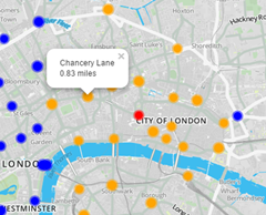 There are tube strikes planned for 25th August 2015 and 28th August 2015 with disruption through the week. The nature of the London Underground means that it is not all obvious that walks between stations can be quite short. This blog post introduces a handy tool to help you work out “Can I walk it?”
You can find the tool here:
To use it start by selecting the station you want to walk from, either by using the “Where am I?” dropdown or by clicking one of the coloured station symbols (or close to it). The map will then refresh, the station you selected is marked by a red disk, the stations within 1.5 miles of the starting station are marked by an orange disk and those more than 1.5 miles away are marked by a blue disk. 1.5 miles is my “walkable” threshold, it takes me about 25 minutes to walk that far. You can enter your own “walkable” threshold in the “I will walk” box and press refresh or select a new starting station to refresh the map.
The station markers will show the station names on mouseover, and the distances to the starting station once it has been selected.
This tool comes with no guarantees, the walking distances are estimated and these estimates may be faulty, particularly for river crossings. Weather conditions may make walking an unpleasant or unwise decision. The tool relies on the user to supply their own reasonable walking threshold. Your mileage may vary.
To give a little background to this project: I originally made this tool using Tableau. It was OK but tied to the Tableau Public platform. I felt it was a little slow and unresponsive. It followed some work I’d done visualising data relating to the London Underground which you can read about here.
As an exercise I thought I’d try to make a “Can I walk it?” web application, re-writing the original visualisation in JavaScript and Python. I’ve been involved with projects like this at ScraperWiki but never done the whole thing for myself. I used the leaflet.js library to provide the mapping, the Flask library in Python to serve the data, Boostrap to make it look okay and Docker containers on Digital Ocean to deploy the application.
The underlying data for this tool comes from Open Street Map, where the locations of all the London Underground stations are encoded as latitude and longitude. With this information in hand it is possible to calculate the distances between stations. Really I want the “walking distance” between stations rather than the crow flies distance which is what this data gives me. Ideally to get the walking distance I’d use Google Directions API but unfortunately this has a rate limit of 2500 calls per day and I need to make about 36000 calls to get all the data I need!
The code is open source and available in this BitBucket repository:
https://bitbucket.org/ian_hopkinson/london-underground-app
Comments and feedback are welcome!
Jul 17 2015
Book review: Docker Up & Running by Karl Matthias and Sean P. Kane
This review was first published at ScraperWiki.
This last week I have been reading  Docker Up & Running by Karl Matthias and Sean P. Kane, a newly published book on Docker – a container technology which is designed to simplify the process of application testing and deployment.
Docker is a very new product, first announced in March 2013, although it is based on older technologies. It has seen rapid uptake by a number of major web-based companies who have open-sourced their tooling for using Docker. We have been using Docker at ScraperWiki for some time, and our most recent projects use it in production. It addresses a common problem for which we have tried a number of technologies in search of a solution.
For a long time I have thought of Docker as providing some sort of cut down virtual machine, from this book I realise this is the wrong mindset – it is better to think of it as a “process wrapper”. The “Advanced Topics” chapter of this book explains how this is achieved technically. This makes Docker a much lighter weight, faster proposition than a virtual machine.
Docker is delivered as a single binary containing both client and server components. The client gives you the power to build Docker images and query the server which hosts the running Docker images. The client part of this system will run on Windows, Mac and Linux systems. The server will only run on Linux due to the specific Linux features that Docker utilises in doing its stuff. Mac and Windows users can use boot2docker to run a Docker server, boot2docker uses a minimal Linux virtual machine to run the server which removes some of the performance advantages of Docker but allows you to develop anywhere.
The problem Docker and containerisation are attempting to address is that of capturing the dependencies of an application and delivering them in a convenient package. It allows developers to produce an artefact, the Docker Image, which can be handed over to an operations team for deployment without to and froing to get all the dependencies and system requirements fixed.
Docker can also address the problem of a development team onboarding a new member who needs to get the application up and running on their own system in order to develop it. Previously such problems were addressed with a flotilla of technologies with varying strengths and weaknesses, things like Chef, Puppet, Salt, Juju, virtual machines. Working at ScraperWiki I saw each of these technologies causing some sort of pain. Docker may or may not take all this pain away but it certainly looks promising.
The Docker image is compiled from instructions in a Dockerfile which has directives to pull down a base operating system image from a registry, add files, run commands and set configuration. The “image” language is probably where my false impression of Docker as virtualisation comes from. Once we have made the Docker image there are commands to deploy and run it on a server, inspect any logging and do debugging of a running container.
Docker is not a “total” solution, it has nothing to say about triggering builds, or bringing up hardware or managing clusters of servers. At ScraperWiki we’ve been developing our own systems to do this which is clearly the approach that many others are taking.
Docker Up & Running is pretty good at laying out what it is you should do with Docker, rather than what you can do with Docker. For example the book makes clear that Docker is best suited to hosting applications which have no state. You can copy files into a Docker container to store data but then you’d need to work out how to preserve those files between instances. Docker containers are expected to be volatile – here today gone tomorrow or even here now, gone in a minute. The expectation is that you should preserve state outside of a container using environment variables, Amazon’s S3 service or a externally hosted database etc – depending on the size of the data. The material in the “Advanced Topics” chapter highlights the possible Docker runtime options (and then advises you not to use them unless you have very specific use cases). There are a couple of whole chapters on Docker in production systems.
If my intention was to use Docker “live and in anger” then I probably wouldn’t learn how to do so from this book since the the landscape is changing so fast. I might use it to identify what it is that I should do with Docker, rather than what I can do with Docker. For the application side of ScraperWiki’s business the use of Docker is obvious, for the data science side it is not so clear. For our data science work we make heavy use of Python’s virtualenv system which captures most of our dependencies without being opinionated about data (state).
The book has information in it up until at least the beginning of 2015. It is well worth reading as an introduction and overview of Docker.
Jul 06 2015
Book Review: Learning Spark by Holden Karau, Andy Konwinski, Patrick Wendell and Matei Zaharia
This post was first published at ScraperWiki.
 Apache Spark is a system for doing data analysis which can be run on a single machine or across a cluster, it is pretty new technology – initial work was in 2009 and Apache adopted it in 2013. There’s a lot of buzz around it, and I have a problem for which it might be appropriate. The goal of Spark is to be faster and more amenable to iterative and interactive development than Hadoop MapReduce, a sort of Ipython of Big Data. I used my traditional approach to learning more of buying a dead-tree publication, Learning Spark by Holden Karau, Andy Konwinski, Patrick Wendell and Matei Zaharia, and then reading it on my commute.
The core of Spark is the resilient distributed dataset (RDD), a data structure which can be distributed over multiple computational nodes. Creating an RDD is as simple as passing a file URL to a constructor, the file may be located on some Hadoop style system, or parallelizing an in-memory data structure. To this data structure are added transformations and actions. Transformations produce another RDD from an input RDD, for example filter() returns an RDD which is the result of applying a filter to each row in the input RDD. Actions produce a non-RDD output, for example count() returns the number of elements in an RDD.
Spark provides functionality to control how parts of an RDD are distributed over the available nodes i.e. by key. In addition there is functionality to share data across multiple nodes using “Broadcast Variables”, and to aggregate results in “Accumulators”. The behaviour of Accumulators in distributed systems can be complicated since Spark might preemptively execute the same piece of processing twice because of problems on a node.
In addition to Spark Core there are Spark Streaming, Spark SQL, MLib machine learning, GraphX and SparkR modules. Learning Spark covers the first three of these. The Streaming module handles data such as log files which are continually growing over time using a DStream structure which is comprised of a sequence of RDDs with some additional time-related functions. Spark SQL introduces the DataFrame data structure (previously called SchemaRDD) which enables SQL-like queries using HiveQL. The MLlib library introduces a whole bunch of machine learning algorithms such as decision trees, random forests, support vector machines, naive Bayesian and logistic regression. It also has support routines to normalise and analyse data, as well as clustering and dimension reduction algorithms.
All of this functionality looks pretty straightforward to access, example code is provided for Scala, Java and Python. Scala is a functional language which runs on the Java virtual machine so appears to get equivalent functionality to Java. Python, on the other hand, appears to be a second class citizen. Functionality, particularly in I/O, is missing Python support. This does beg the question as to whether one should start analysis in Python and make the switch as and when required or whether to start in Scala or Java where you may well be forced anyway. Perhaps the intended usage is Python for prototyping and Java/Scala for production.
The book is pitched at two audiences, data scientists and software engineers as is Spark. This would explain support for Python and (more recently) R, to keep the data scientists happy and Java/Scala for the software engineers. I must admit looking at examples in Python and Java together, I remember why I love Python! Java requires quite a lot of class declaration boilerplate to get it into the air, and brackets.
Spark will run on a standalone machine, I got it running on Windows 8.1 in short order. Analysis programs appear to be deployable to a cluster unaltered with the changes handled in configuration files and command line options. The feeling I get from Spark is that it would be entirely appropriate to undertake analysis with Spark which you might do using pandas or scikit-learn locally, and if necessary you could scale up onto a cluster with relatively little additional effort rather than having to learn some fraction of the Hadoop ecosystem.
The book suffers a little from covering a subject area which is rapidly developing, Spark is currently at version 1.4 as of early June 2015, the book covers version 1.1 and things are happening fast. For example, GraphX and SparkR, more recent additions to Spark are not covered. That said, this is a great little introduction to Spark, I’m now minded to go off and apply my new-found knowledge to the Kaggle – Avito Context Ad Clicks challenge!
Jul 05 2015
Portinscale 2015
We had an abortive trip to Portinscale in the Lake District for our summer holiday last year, ended prematurely by illness. This year we’re back and have improved greatly on last years performance! Portinscale is just outside Keswick, a small town at the head of Derwentwater. In the past we would have stayed a little further from civilisation so we could go for longish walks from the door but with 3 year old Thomas a bunch of attractions in easy distance is preferable.
Day 1 – Sunday
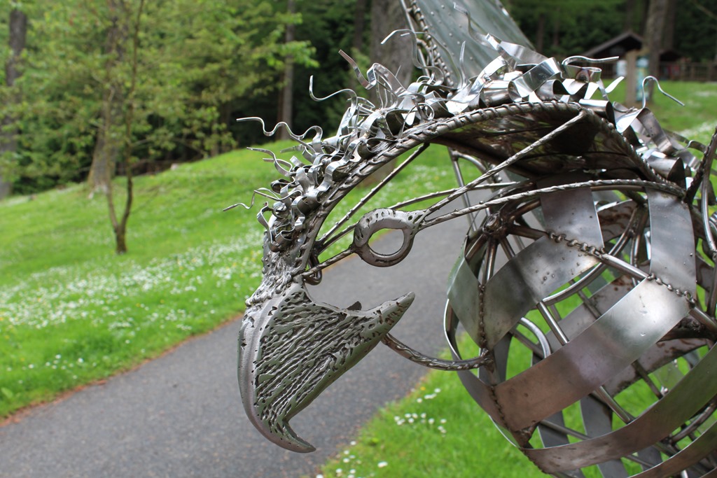
Rather than fit packing and driving the relatively short distance to Portinscale from Chester into a day, whilst simultaneously meeting the arrival time requirements, we travelled up on Sunday morning. In the afternoon we went to Whinlatter Forest Park, a few miles up the road. The entrance is guarded by a fine sculpture of an osprey.
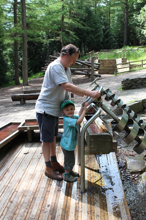
It has an extensive collection of trails for pedestrians and cyclists. A Go Ape franchise for people who like swinging from trees, some Gruffalo / Superworm themed trails for children. And a wild play area featuring Thomas’ favourite thing – a pair of Archimedes Screws:
There’s also a very nice cafe. We visited Whinlatter several times of an afternoon.
Day 2 – Monday
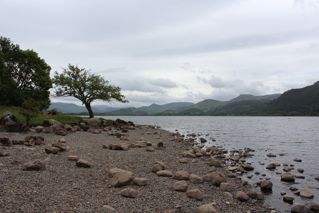
We went to Mirehouse in the morning, a lakeside estate with a smallish garden and a rather pleasant walk down to Bassenthwaite Lake.
There’s a fine view from the lake down towards Keswick.
In the afternoon we went to the Pencil Museum in Keswick, not a large attraction but Thomas liked Drew the giant and we got 5 pencils for an outlay of £3.
Day 3 – Tuesday
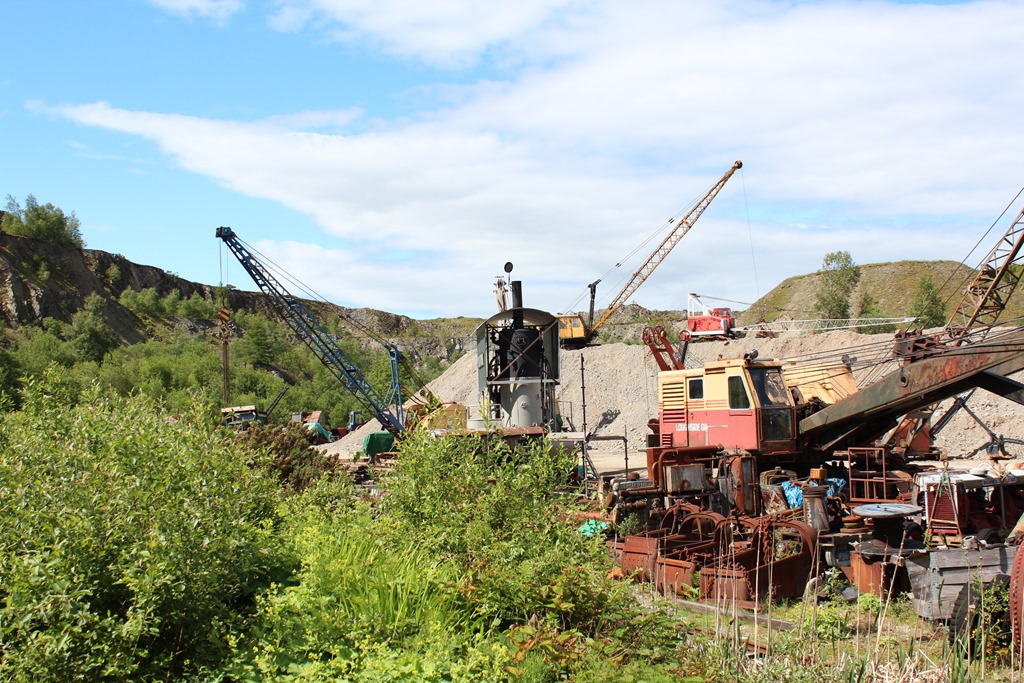
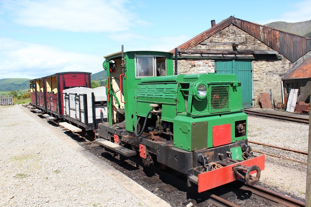
In the morning we went to Threlkeld Mining Museum. Its full of cranes and various bits of mining machinery from the past 100 years or so. There is a narrow gauge railway line which runs half a mile or so to the head of the quarry from the visitor centre. Threlkeld is not a slick affair but it is great fun for a small child fond of cranes, and the volunteers are obviously enthused by what they are doing. To be honest, I’m rather fond of industrial archaeology too!
Basically, they collect cranes.
All of which are in some degree of elegant decay
For our visit they were running a little diesel train:
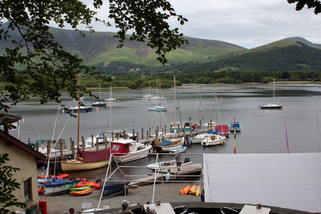
In the afternoon we walked down to Nichols End, a marina on Derwentwater close by our house in Portinscale.
Day 4 – Wednesday
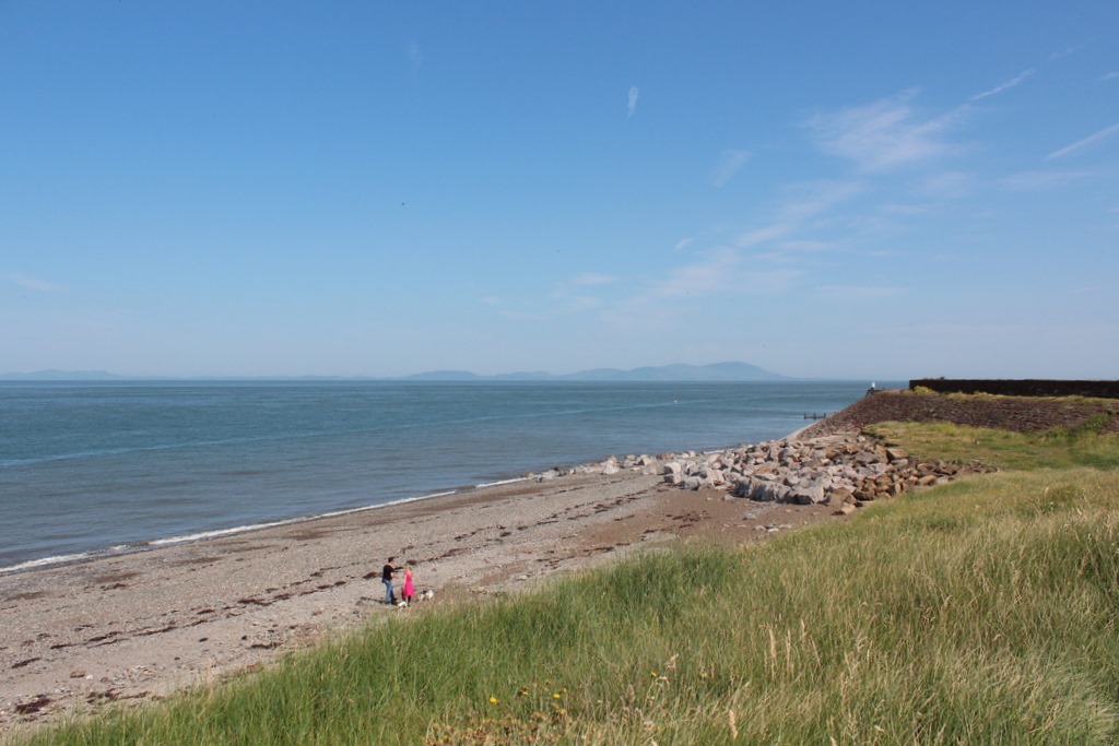
My records show that we last visited Maryport 15 years ago. It has the benefit of being close to Keswick – only half an hour or so away. We enjoyed a brief paddle in the sea, on a beach of our own before heading to the small aquarium in town.
Whinlatter Forest Park once again in the afternoon.
Day 5 – Thursday
On leaving the house we thought we would be mooching around Keswick whilst our car was being seen to for “mysterious dripping”, as it was Crosthwaite Garage instantly diagnosed an innocuous air conditioning overflow. So we headed off to Lodore Falls, alongside Derwentwater before returning to Hope Park in Keswick.
Thomas declared the gently dripping woods on the way to Lodore Falls to be “amazing”:
The falls themselves are impressive enough, although the view is a little distant when you are with a small child, who coincidently loves waterfalls and demands their presence on every walk:
Hope Park was busy, but it is a pretty lakeside area with formal gardens and golf a little back from the shore.
In the afternoon we visited Dodd Wood, which is just over the road from Mirehouse, where we did a rather steep walk.
Day 6 – Friday
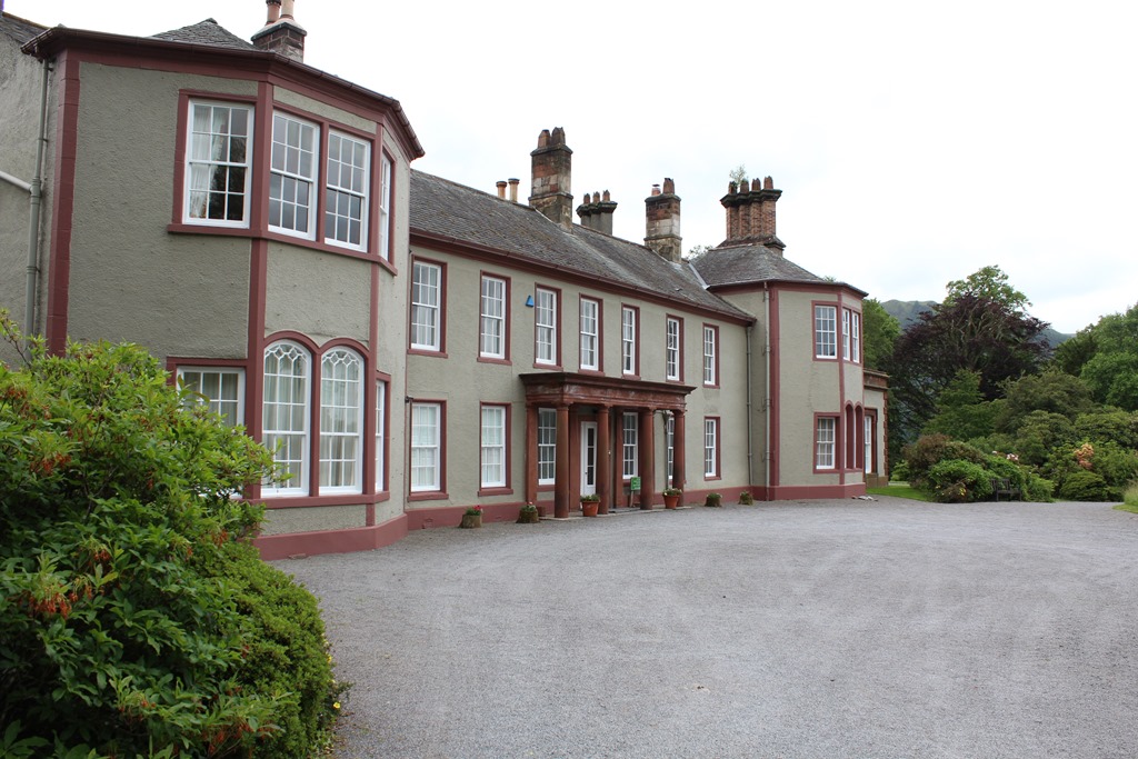
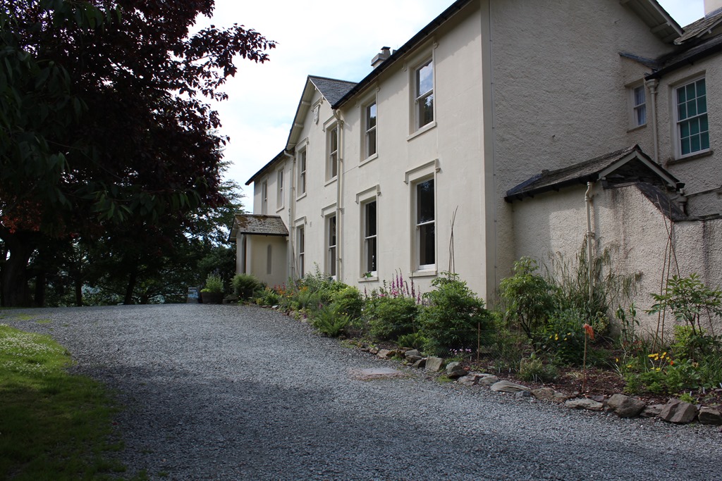
On our final day we visited Allan Bank in Grasmere, this is a stealth National Trust property, formerly home to William Wordsworth and one of the founders of the National Trust, Canon Rawnsley. “Stealth” because it is barely advertised or sign posted, and is run in manner far more relaxed than any other National Trust place I’ve visited. It’s a smallish house:
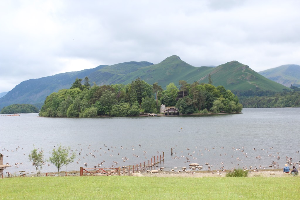
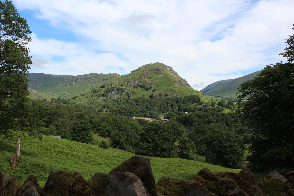
With glorious views:
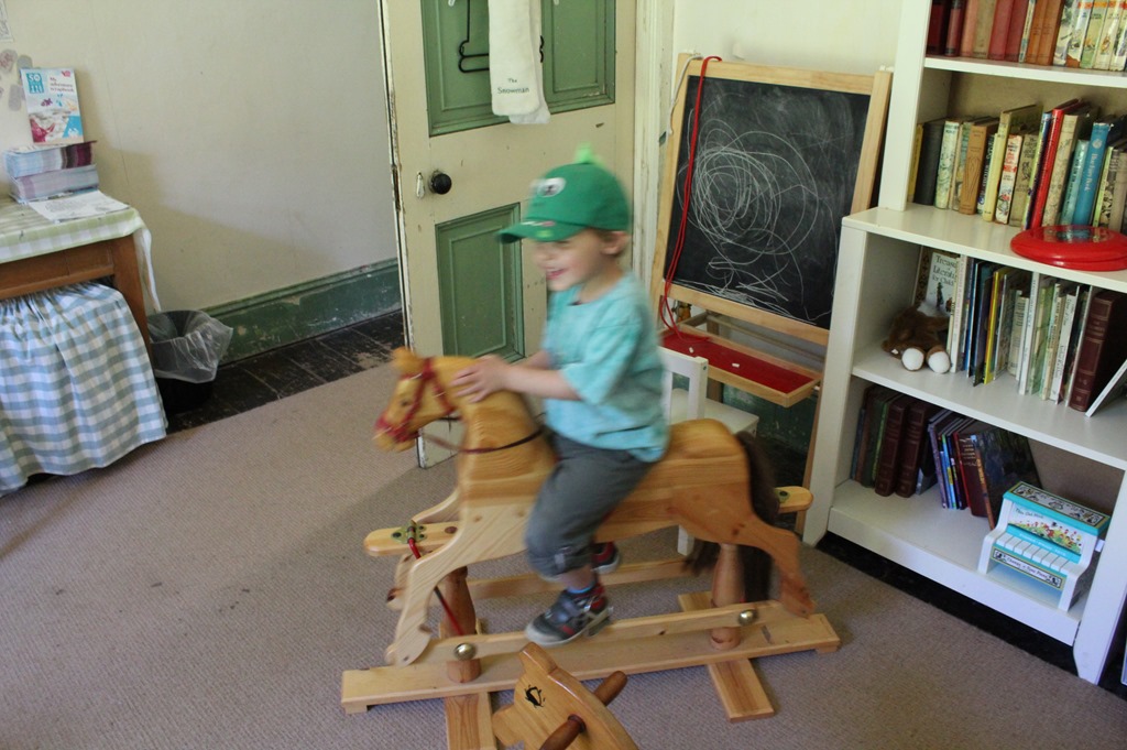
The house was damaged by fire a few years ago, and has only really been refurbished in as far as making it weather proof. Teas and coffees are available on unmatching crockery for a donation (you pay for cake though), and you’re invited to take them where you please to drink. There is a playroom ideally suited to Thomas’ age group, along with rooms Wordsworth and Rawnsley occupied upstairs.
It has the air of a hippy commune, and it’s sort of glorious.
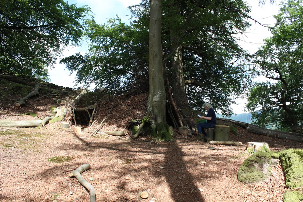
Outside the grounds are thickly wooded on a steep slope, there is a path approximately around the perimeter which takes in the wild woods, several dens and some lovely views.
We glimpsed a red squirrel in the woods.
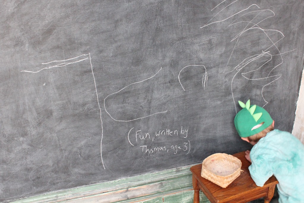
As Thomas wrote, it was "”Fun”!
In the afternoon a final trip to Whinlatter Forest Park.
We left on Saturday amidst heavy early morning rain, the only serious daytime rain of the holiday – probably the best week of weather I’ve had in the Lake District!

