Author's posts
Aug 14 2020
Book review: Your voice speaks volumes by Jane Setter
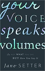 I have a habit of reading the books written by people I follow on Twitter, Your voice speaks volumes by Jane Setter falls into that category. It is a book about how we speak (if we speak English, and largely if we are British).
Your voice is divided into seven chapters which cover seven separate themes.
It starts with a description of the mechanics of speech, and how we annotate sounds. I particularly like the chart of when children typically manage to produce different sounds, the earliest part of English come between 18 months and two years of age, with the last appearing between 5 and 8. I dutifully touched my larynx to feel the difference between the voiceless /s/ and the voiced /z/. Setter underestimates my ignorance by not explaining the difference between vowels and constants – I can tell you which letters are vowels but not why those letters are vowels.
The second chapter on accents is the one I found most fascinating, it turns out that certain features of accents follow the lines of the Anglo-Saxon occupation of Britain. So called rhotic, and non-rhotic pronunciation. Coming from the West Country my accent is probably a bit rhotic – I pronounce r’s more strongly. It is interesting to see accents cross a thousand years. This chapter also talks about how we are judged by our accents, a recurring theme is that women are more often criticised for their voices.
Chapter three talks about how we make judgements of a person based on the basis of how they speak, and how we might try to change those perceptions. Here we get an anecdote about Setter’s partner at university who had a masculine voice that did not match his slight physique! As in the previous chapter it is women who get the brunt of criticism for being perceived to have changed their voices. Men struggle to change their voices to sound more masculine/sexy – this is probably an evolutionary side effect – a voice indication of fitness that could be faked would not be very helpful. Included in this chapter are “uptalk” and vocal fry, uptalk is lifting the intonation at the end of a sentence. Uptalk I understand, I always associate it with Australians. Vocal fry is probably best understood by search youtube, it makes me think of Britney Spears.
I was shocked to discover that actors are still expected to have “received pronunciation RP” as their default voice and the ability to do General American as a “second language”. This is reflected in newsreaders where accents are largely notable by their absence. The chapter starts with some comments about Alesha Dixon singing “God Save the Queen”, she was criticised, purportedly, for Americanising her pronunciation by certain sections of the press. Setter highlights that Dixon’s pronunciation is only slightly Americanised and is most likely as a result of background in R&B music. It is an unwritten rule that different styles of music conventionally are sung in different accents, Country music and R&B “sound” better with an American accent. Hence bands like The Rolling Stones often have vocals with a hint of an American accent. Singing is a performance, rather than speech and so singers tend to learn a song, accent and all rather than sing with their speaking voice.
The chapter on forensic speaker analysis, based on Setters work in court this divides into auditory analysis, done with the ear, focused on the larger scale features of the voice and acoustic analysis which is done using software and looks at the frequency spectrum. It was interesting to learn how voice line-ups are constructed. The message of this chapter is that voice matches tend are indicative rather than absolute, analysis can show that two voice recordings could be from the same speaker but not confirm that fact.
The penultimate chapter talks about the importance of voice to the transgender community, to a degree trans men have an easier job, taking testerone leads to a natural lowering of the voice but the same is not true in reverse for trans women. Although pitch is the primary discriminating feature between male and female voices, it is not the only one.
The book finishes with a chapter on English as a second language. Setter has worked with call centre staff from India to help them provide a better service. Some of the complaints about such call centre staff boil down simply to customers not wanting to speak to foreigners. But in other cases the way in which English is spoken in England and India leads to misunderstanding in the manner of a conversation. What to an Indian English speaker is normal may sound like annoyance or frustration to an Indian speaker which makes me think of The Culture Map by Erin Meyer.
Your voice is written in quite a chatty style with a number of anecdotes to move the story along. It provides a useful overview of at least part of the work of a phonetician. The accompanying web page is a bit sparse (here) but includes a PDF of the introduction, so you can try before you buy. Your voice is endorsed by David Crystal whose books on the English language I feel I grew up on – to be honest I was pleased to discover he was still alive!
Aug 01 2020
Book review: 1491 by Charles C. Mann
 I read 1491: New revelations of the Americas before Columbus by Charles C. Mann as a follow up to How the States got their Shapes by Mark Stein. I had been frustrated at how this latter book had focussed on the colonial period, with native Americans almost completely elided.
The book tracks through three broad themes looking at those themes as they relate to Amazonia in the South, through Peru into central America and then into North America. The emphasis is around central America and the more northern parts of South America. I think this is a result of where the archaeology are found.
The first theme is the numbers of native Americans in the time before colonisation, the broad picture here is that the population was large prior to colonisation, and in places still high as colonisation started but it was reduced dramatically by disease brought by the colonists – figures as high as a 90% reduction are discussed. The native Americans were highly vulnerable to the diseases the Europeans brought, both because they were genetically less diverse than the Europeans, and they had never experienced anything like the diseases brought. Initial contact between Europeans and Americans took place in the 16th century, with more serious attempts at colonisation not getting under way for a century, by which point disease had taken its toll. In an appendix Mann discusses whether syphilis travelled to Europe from the Americas, the evidence here is not clear.
The European view of the pre-colonial population of the Americas has varied, with the initial explorers recognising the sizeable populations of in the lands they found but as colonisation continued those memories were lost as the native population plummeted. Furthermore it was in the interests of the colonists to see the Americas as empty land, rather than land they took from others. During the 20th century these views have slowly been revised although there is considerable debate over exactly the scale of death through disease.
The second theme is origins: when were humans first found in the Americas? During the early part of the 20th century the view developed that the first human settlers in the Americas arrived over a land bridge from Asia around 15,000 years ago – the so called Clovis people. Towards the end of the 20th century this view has been revised with earliest origins going back to 30,000 or so years ago. In any case there were significant civilisations leaving behind ruins and burials dating back to 7,000 years ago.
The final theme is landscape, to what degree is the landscape we see in the Americas human-made? Here it seems that Europeans have one view of a human-made landscape which does not match what is found in the Americas. The Americas are the origin to a huge variety of important agricultural crops (potatoes, maize, peppers, cassava/manioc and squashes) but they are not found in the fields associated with European agriculture but more in cultivated woodland. This dichotomy is perhaps starkest in Amazonia where there is still considerable dispute as to what civilisations once lived there, if any, and to what degree the Amazonian rainforest is human-made. Again this is tinged with modern European and colonial sentiments, in particular from a conservationist point of view it is preferable to see the Amazon as an untouched wilderness rather than a landscape shaped by humans since this provides a strong argument against allowing (renewed) development.
American cities both North and South were often different from European cities, commerce has always been important in European cities but in the Americans cities were often great ritual centres with living accommodation for farmers and other workers but little sign of trade.
In a coda Mann discusses the potential impact that the egalitarian Haudenosaunee alliance had on the founding fathers of the United States. Mann is clear that his view on this is not yet mainstream but highlights that principles of the founding fathers were closer to those of the Haundenosaunee than those of the class-based hierarchy of European countries. Early colonists had extensive interactions with the native Americans, and it wasn’t unknown for them to join their communities seeing them as more congenial than their own.
The book finishes with appendices on names, the khipu system of writing with knots, syphilis and the Mesoamerican calendars. I must admit I bristled early on at the use of the term “Indian”, rather than “native American” but as Mann highlights “Indians” usually use the term “Indian” themselves without objection in the relevant context and he uses “Indian” and “native American” interchangeable simply to introduce a degree of variety. More generally he attempts to use the name that a member of a group would prefer to use for that group. It parallels my preference to be called European, British, English, from Dorset or from Cheshire depending on context.
I must admit I was aiming for a book that covered North American pre-colonial history in more detail. That said 1491 is readable, covering a great deal of ground. My next step is probably to look for a history of the Haudenosaunee.
Jul 07 2020
Type annotations in Python, an adventure with Visual Studio Code and Pylance

I’ve been a Python programmer pretty much full time for the last 7 or 8 years, so I keep an eye out for new tools to help me with this. I’ve been using Visual Studio Code for a while now, and I really like it. Microsoft have just announced Pylance, the new language server for Python in Visual Studio Code.
The language server provides language-sensitive help like spotting syntax errors, providing function definitions and so forth. Pylance is based on the type checking engine Pyright. Python is a dynamically typed language but recently has started to support type annotations. Dynamic typing means you don’t tell the interpreter what “type” a variable is (int, string and so forth) you just use it as such. This contrasts with statically typed languages where for every variable and function you define a type as you write your code. Type annotations are a halfway house, they are not used by the Python interpreter but they can be used by tools like Pylance to check code, making it more likely to run correctly on first go.
Pylance provides a range of “Intellisense” code improvement features, as well as type annotation based checks (which can be switched off).
I was interested to use the type annotations checking functionality since one of the pleasures of working with statically typed languages is that once you’ve satisfied your compiler that all of the types are right then it has a better chance of running correctly than a program in a dynamically typed language.
I will use the write_dictionary function in my little ihutilities library as an example here, this function is defined in the file io_utils.py. The appropriate type annotation for write_dictionary is:
def write_dictionary(filename: str, data: List[Dict[str,Any]],append:Optional[bool]=True, delimiter:Optional[str]=",") -> None:
Essentially each variable is followed by a colon, and then a type (i.e str). Certain types are imported from the typing library (Any, List, Optional and Dict in this instance). We supply the types of the elements of the list, or dictionary. The Any type allows for any type. The Optional keyword is used for optional parameters which can have a default value. The return type is put at the end after the ->. In a *.pyi file described below, the function body is replaced with ellipsis (…).
Actually the filename type hint shouldn’t be string but I can’t get the approved type of Union[str, bytes, os.PathLike] to work with Pylance at the moment.
As an aside Pylance spotted that two imports in the io_utils.py library were unused. Once I’d applied the type annotation to the function definition it inferred the types of variables in the code, and highlighted where there might be issues. A recurring theme was that I often returned a string or None from a function, Pylance indicated this would cause a problem if I tried to measure the length of None.
There a number of different ways of providing typing information, depending on your preference and whether you are looking at your own code, or at a 3rd party library:
- Types provided at definition in the source module – this is the simplest method, you just replace the function def line in the source module file with the type annotated one;
- Types provided in the source module by use of *.pyi files – you can also put the type-annotated function definition in a *.pyi file alongside the original file in the source module in the manner of a C header file. The *.pyi file needs to sit in the same directory as its *.py sibling. This definition takes precedence over a definition in the *.py file. The reason for using this route is that it does not bring incompatible syntax into the *.py files – non-compliant interpreters will simply ignore *.pyi files but it does clutter up your filespace. Also there is a risk of the *.py and *pyi becoming inconsistent;
- Stub files added to the destination project – if you import write_dictionary into a project Pylance will highlight that it cannot find a stub file for ihutilities and will offer to create one. This creates a `typings` subdirectory alongside the file on which this fix was executed, this contains a subdirectory called `ihutilities` in which there are files mirroring those in the ihutilities package but with the *.pyi extension i.e. __init__.pyi, io_utils.py, etc which you can modify appropriately;
- Types provided by stub-only packages – PEP-0561 indicates a fourth route which is to load the type annotations from a separate, stub only, module.
- Types provided by Typeshed – Pyright uses Typeshedfor annotations for built-in and standard libraries, as well as some popular third party libraries;
Type annotations were introduced in Python 3.5, in 2015, so are a relatively new language feature. Pyright is a little over a year old, and Pylance is a few days old. Unsurprisingly documentation in this area is relatively undeveloped. I found myself looking at the PEP (Python Enhancement Proposals) references as often as not to understand what was going on. If you want to see a list of relevant PEPs then there is a list on the Pyright README.md, I even added one myself.
Pylance is a definite improvement on the old Python language server which was itself more than adequate. I am currently undecided about type annotations, the combination of Pylance and type annotations caught some problems in my code which would only come to light in certain runtime circumstances. They seem to be a bit of an overhead which I suspect I would only use for frequently used library routines, and core code which gets run a lot and is noticeable by others when it fails. I might start by adding in some *.pyi files to my active projects.
Jun 07 2020
Book review: Science City by Alexandra Rose and Jane Desborough
 On Twitter I hang out with a load of historians of science, and this has lead me to Science City: Craft, Commerce and Curiosity in London 1550-1800 by Alexandra Rose and Jane Desborough. This is an edited volume which accompanies the new Linbury Gallery at the Science Museum, combining objects from the Science Museum, King George III collection and the Royal Society. This book touches on many of the books I’ve read previously on the Board of Longitude, the transit of Venus, surveying and map making.
The main part of the book is four roughly chronological chapters covering the development of an instrument making industry in London, the Royal Society, public displays of science, and global expeditions. At the beginning of the period covered by the book, 1550, London was not a particularly notable city – it was a quarter the size of Paris and only twice the size of Norwich – England’s second city at the time. It had no universities, in fact it wasn’t to have a university until 1826.
The instrument trade in London started with a need to fulfil the requirement for “mathematical instruments” for surveying, gunnery and architecture. It was boosted by immigrants from the Low Countries fleeing persecution. In 1571 5% of the London population were “strangers” – born outside of England. These immigrants were not unwelcome, foreign manufactured goods were often seen as better quality which caused some resentment in the Guilds. Skills were developed and maintained by apprenticeships. These were typically found by personal contacts in the 16th century, there was no advertising of positions. Science City traces some apprenticeship “lineages”. In the early days there was no specific Guild for instrument making.
The second chapter brings in the Royal Society founded in 1666. As well as the instrumental needs of Robert Hooke, its Curator of Experiments, it stimulated a wider trade in instruments. The members of the Royal Society were keen to replicate experiments, or do their own experiments to share with the Society (or at least keen enough to spend money on instruments). Variants of the air pump demonstrations Hooke did were still being done 40 years later. The Royal Society put London at the centre of a network of scientific correspondents, and to some degree defined the way to be a scientist that maintains to this day.
In the ensuing years public science became a popular entertainment. Popularisers of science needed instruments to ply their trade. By this point in the first half of the 18th century there are 300 instrument makers in London, their business is divided into mathematical instruments (theodolites, sextants and the like), optical instruments (microscopes and telescopes) and philosophical instruments (those used to demonstrate physical principles). Its interesting to see the birth of branding at this point, makers were known by their shops signs and for clarity they would typically use a consistent image across there pamphlets and shopfront (rather than simply words). Examples include Benjamin Martin’s “spectacle” logo, and Edward Culpeper’s crossed daggers.
The final chapter covers the second half of the 18th century, this is at a time where the Ordnance Survey is founded alongside triangulation surveys with France. The chapter speaks to the global reach of London in trade and in science. This is the time of the Board of Longitude which was founded, making its major awards to John Harrison for his chronometer in the second half of the 18th century. The expeditions to view the transit of Venus in 1769 were also significant – the Royal Society petitioned the King to fund an expedition to Tahiti, this was accompanied by other expeditions which led to a requirement for moderately standardised instrumentation to make the measurements. London was able to supply this demand.
Science City finishes with interviews with an instrument maker (Joanna Migdal), the President of the Royal Society and the Lord Mayor of London (also a trustee of the Science Museum). The first of these I found really interesting I wish there were photos of the sundials the interviewee made, you can find some here on their website. Migdal’s work, individual, handcrafted items, is probably in the character of the instrument making of this book but differs from the typical instrument ecosystems these days.
The book is rather smaller than I expected but it is beautifully illustrated, more a bedside table than a coffee table book. I enjoy these catalogues of museum exhibitions more than the exhibitions themselves. In the gallery you are pushed for time and space, reading the descriptions can be difficult cross-referencing to other things you have read is impractical. A book makes it a more comfortable process but just lacks the immediacy of seeing the objects “in-person”.
May 30 2020
Gear review: Boss RC-3 Loop station
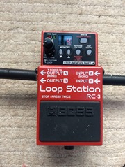 In a change from usual service I am reviewing some guitar related gear: a Boss RC-3 Loop Station. Review is probably not the right word, this is the only guitar pedal of this type I’ve used so really this is more about describing what it does, which would be useful for other novices, capturing some of the instructions in a more readable form and sharing some resources.
A loop pedal is a device which records sound – pedals are devices designed to be activated with a foot. The intention of a loop pedal is to capture short sequences of sound which you then play over as they repeat in the background, so that one musician can make the sound of many. Ed Sheeran and KT Tunstall are particularly well-known users of the loop pedal, needless to say that despite owning one I sound no where near as good!
It’s worth noting that although this is advertised as a guitar pedal it will record any sound fed into the input side, I’ve used it with my electric drum kit, it will work with the keyboards we have and if I had a microphone I could sing into it (but nobody wants that).
There are plenty of loop pedals around, following a series of price points / sizes.The cheapest one in the Boss range is the RC-1 for something like £80, I paid £125 for the RC-3 which is one step up from the most basic models. Above the RC-3 in the Boss range are the RC-30 for £171 which has two large size foot switches and the RC-300 for £440 which is much larger and has footswitches for each of three tracks.
The RC-3 has 99 slots to record loops to, and will provide a rhythm track as well in one of 9 styles. There is a USB port which presents the pedal as a file directory, this allows you to backup your loops and save WAV files from elsewhere to it. I picked the Boss because I have a couple of other Boss devices (my amplifier and expression pedal) and I like the brand.
The device itself is nice and chunky, made out of metal. I think I prefer the big rubberised pedal style to the round metal push buttons found on other loop pedals. I found the other controls a bit small and fiddly, I’m not as young as I used to be – bending down and looking at small things are hard! Fundamentally this is a “small format device” problem which isn’t limited to the Boss pedal, space is limited to control the functionality provided so you get a two character display and five push buttons.
The buttons select the memory slot to be used (or cycle through options), select the rhythm functionality, write a loop to a memory slot and allow you to set the tempo of the rhythm track.
A couple of handy hints I picked up from this video by Reidy’s – a fine Lancashire company: firstly the default mode is that pedal presses take you from record to overdub to playback modes, you can change this to record to playback to overdub by holding down the tempo button whilst switching the device on. As a beginner this feels more natural. Secondly, you can clear, undo and redo the current loop by long presses on the pedal – so you can muck around recording and deleting little phrases with just the foot control. These features are both explained in the paper manual which comes with the device.
You can also change the record mode from the default, of starting recording as soon as the pedal is pressed, to auto recording which starts when you start playing and count-in which sounds the rhythm for a measure before recording starts.
The built-in rhythms are as follows:
- Hi-hat
- Kick & Hi-hat
- Rock 1
- Rock 2
- Pop
- Funk
- Shuffle
- R&B
- Latin
- Percussion
The tempo is set by tapping the tempo button, you can’t fix it to a specific value using the up and down buttons – most likely because the display can only handle a two digit tempo – and that’s a bit small.
One thing worth noting is if you have a Boss Katana 50 and an expression pedal you will not hear the effect of the expression pedal on the loop pedal recording. This is because the loop pedal is not seeing the expression pedal in its input. You can sort of capture it by putting the loop pedal on the output side of the Katana and plugging headphones, or another amplifier, into the loop pedal but it is not an ideal solution. Higher specification Boss Katana have an external effects loop which is where you would put the loop pedal. More generally the effects you hear on playback are the ones set on the amplifier at playback time, not those being used at record time.
Applications
I’ve already used the Boss for the following:
- Fiddling about with amplifier tone – record a loop then adjust amplifier settings as it plays back – you don’t have to wrangle your guitar and amplifier at the same time and can hear immediately the effect of your knob twiddling;
- Record your practicing – I use Yousician which has a lot of exercises – chords changes, fingerpicking, scales and the like. The loop pedal is an easy way to do a quick recording to hear where you are going wrong;
- Simple rhythm track – it has a bunch of rhythm styles whose tempo you can adjust;
- Backing chords to play over – I need to practice doing this;
- Backing sounds from elsewhere
Summary
I am pleased with my purchase! I think it will take me quite a while to get to grips with recording a backing loop – I’ve been watching the Justin Guitar videos below to help me with this.
Resources
- Justin Guitar – loop pedal overview – 20 minutes on how to use any loop pedal
- Justin Guitar – Shape of you lesson
- Paul Davids – 7 fun guitar looping songs – more on what you should loop rather than how
- Reidy’s How to use a looper guide – specific to the RC-3

