Book review: A history of the world in twelve maps by Jerry Brotton

HistoryOfTheWorldInTwelveMapsAs a fan of maps, I was happy to add A History of the World in Twelve Maps by Jerry Brotton to my shopping basket (I bought it as part of a reduced price multi-buy deal in an actual physical book shop).

A History traces history through the medium maps, various threads are developed through the book: what did people call the things we now call maps? what were they trying to achieve with their maps? what geography was contained in the maps? what technology was used to make the maps?

I feel the need to explicitly list, and comment on, the twelve maps of the title:

1. Ptolemy’s Geography 150 AD, distinguished by the fact that it probably contained no maps. Ptolemy wrote about the geography of the known world in his time, and amongst this he collated a list of locations which could be plotted on a flat map using one of two projection algorithms. A projection method converts (or projects) the real life geography of the spherical earth onto the 2D plane of a flat map. Project methods are all compromises, it is impossible to simultaneously preserve relative directions, areas and lengths when making the 3D to 2D transformation. The limitation of the paper and printing technology to hand meant that Ptolemy was not able to realise his map. Also the relatively small size of the known world meant that projection was not a pressing problem. The Geography exists through copies created long after the original was written.

2. Al-idrisi’s Entertainment, 1154AD. The Entertainment is not just a map, it is a description of the world as it was known at the time. This was the early pinnacle in terms of the realisation of the roadmap laid out by Ptolemy. Al-Idrisi, a Muslim nobelman, made the Entertainment for a Christian Sicilian king. It draws on both Christian and Muslim sources to produce a map which will look familiar to modern eyes (except for being upside down). There is some doubt as to exactly which map was included in the Entertainment since no original intact copies exist.

3. Hereford Mappamundi, 1300AD this is the earliest original map in the book but in many ways it is a step backward in terms of the accuracy of its representation of the world. Rather than being a geography for finding places it is a religious object placing Jerusalem at the top and showing viewers scenes of pilgrimage and increasing depravity as one moves away from salvation. It follows the T-O format which was common among such mappmundi.

4. Kangnido world map, 1402AD. To Western eyes this is a map from another world: Korea, again it only exists in copies but not that distant from the original. Here we see strongly the influence of the neighbouring China. The map is about administration and bureaucracy (and contains errors thought to have been added to put potential invaders off the scent). An interesting snippet is that the Chinese saw the nonogram (a square made of 9 squares) as the perfect form – in a parallel with the Greek admiration for the circle. The map also contains elements of geomancy, which was important to the Koreans.

5. Waldseemuller world map, 1507AD. This is the first printed map, it hadn’t really struck me before but printing has a bigger impact than simply price and availability when compared to manuscripts. Printed books allow for all sorts of useful innovations such as pagination, indexes, editions and so forth which greatly facilitate scholarly learning. With manuscripts stating that something is on page 101 of you handwritten manuscript is of little use to someone else with his handwritten copy of the same original manuscript. The significance of the Waldseemuller map is that it is the first European map to name America, it applies the label to the south but it is sometimes seen as the “birth certificate” of the USA. Hence the US Library of Congress recently bought it for $10 million.

6. Diogo Ribeiro, world map, 1529AD. A map to divide the world between the Spanish and Portuguese, who had boldly signed a treaty dividing the world into two hemispheres with them to own one each. The problem arose on the far side of the world, where it wasn’t quite clear where the lucrative spice island of Moluccas lay.

7. Gerard Mercator world map, 1569AD. I wrote about Mercator a while back, in reviewing The World of Gerard Mercator by Andrew Taylor. The Mercator maps are important for several reasons, they introduce new technology in the form of copperplate rather than woodcut printing, copperplate printing enables italic script, rather than the Gothic script that is used in woodcut printing; they make use of the newly developed triangulation method of surveying (in places); the Mercator projection is one of several methods developed at the time for placing a spherical world onto a flat map – it is the one that maintained – despite limitations.And finally he brought the Atlas to the world – a book of maps.

8. Joan Blaeu Atlas maier, 1662. Blaeu was chief cartography for the Dutch East India Company (VOC), and used the mapping data his position provided to produce the most extravagant atlases imaginable. They combined a wide variety of previously published maps with some new maps and extensive text. These were prestige objects purchased by wealthy merchants and politicians.

9. Cassini Family, map of France, 1793. The Cassini family held positions in the Paris Observatory for four generations, starting in the late 17th Century when the first geodesic studies were conducted, these were made to establish the shape of the earth, rather than map it’s features. I reviewed The Measure of the Earth  by Larry D. Ferriero which related some of this story. Following on from this the French started to carry systematic triangulation surveys of all of France. This was the first time the technique had been applied at such scale, and was the forbearer to the British Ordnance Survey, the origins of which are described in Map of a Nation by Rachel Hewitt. The map had the secondary effect of bringing together France as a nation, originally seen by the king as a route to describing his nation (and possibly taxing it), for the first time Parisian French was used to describe all of the country and each part was mapped in an identical manner.

10. The Geographical Pivot of History, Halford Mackinder, 1904. In a way the Cassini map represents the pinnacle of the technical craft of surveying. Mackinder’s intention was different, he used his map to persuade. He had long promoted the idea of geography as a topic for serious academic study and in 1904 he used his map to press his idea of central Asia as being central to the politics and battle for resources in the world. He used a map to present this idea, its aspect and details crafted to reinforce his argument.

11. The Peters Projection, 1973. Following the theme of map as almost-propaganda the Peters projection – an attempted equal-area projection – shows a developing world much larger than we are used to in the Mercator projection. Peters attracted the ire of much of the academic cartographic communities, partly because his projection is nothing new but also because he promoted it as being the perfect, objective map when, in truth it was nothing of the kind. This is sort of the point of the Peters projection, it is open to criticism but highlights that the decisions made about the technical aspects of a map have a subjective weight. Interestingly, many non-governmental organisations took to using the Peters projection because it served their purpose of emphasising the developing world.

12. Google Earth, 2012. The book finishes with a chapter on Google Earth, initially on the technical innovations required to make such a map but then moving on to the wider commercial implications. Brotton toys with the idea that Google Earth is somehow “other“ from previous maps in its commercial intent and the mystery of its methods, this seems wrong to me. A number of the earlier maps he discusses were of limited circulation and one does not get the impression that methods were shared generously. Brotton makes no mention of the Openstreetmap initiative that seems to address these concerns.

In the beginning I found the style of A History a little dry and academic but once I’d got my eye in it was relatively straightforward reading. I liked the broader subject matter, and greater depth than some of my other history of maps reading.

Making a ScraperWiki view with R


This post was first published at ScraperWiki.

In a recent post I showed how to use the ScraperWiki Twitter Search Tool to capture tweets for analysis. I demonstrated this using a search on the #InspiringWomen hashtag, using Tableau to generate a visualisation.

Here I’m going to show a tool made using the R statistical programming language which can be used to view any Twitter Search dataset. R is very widely used in both academia and industry to carry out statistical analysis. It is open source and has a large community of users who are actively developing new libraries with new functionality.

Although this viewer is a trivial example, it can be used as a template for any other R-based viewer. To break the suspense this is what the output of the tool looks like:

R-view

The tool updates when the underlying data is updated, the Twitter Search tool checks for new tweets on an hourly basis. The tool shows the number of tweets found and a histogram of the times at which they were tweeted. To limit the time taken to generate a view the number of tweets is limited to 40,000. The histogram uses bins of one minute, so the vertical axis shows tweets per minute.

The code can all be found in this BitBucket repository.

The viewer is based on the knitr package for R, which generates reports in specified formats (HTML, PDF etc) from a source template file which contains R commands which are executed to generate content. In this case we use Rhtml, rather than the alternative Markdown, which enables us to specify custom CSS and JavaScript to integrate with the ScraperWiki platform.

ScraperWiki tools live in their own UNIX accounts called “boxes”, the code for the tool lives in a subdirectory, ~/tool, and web content in the ~/http directory is displayed. In this project the http directory contains a short JavaScript file, code.js, which by the magic of jQuery and some messy bash shell commands, puts the URL of the SQL endpoint into a file in the box. It also runs a package installation script once after the tool is first installed, the only package not already installed is the ggplot2 package.


function save_api_stub(){
scraperwiki.exec('echo "' + scraperwiki.readSettings().target.url + '" > ~/tool/dataset_url.txt; ')
}
function run_once_install_packages(){
scraperwiki.exec('run-one tool/runonce.R &> tool/log.txt &')
}
$(function(){
save_api_stub();
run_once_install_packages();
});

view raw

code.js

hosted with ❤ by GitHub

The ScraperWiki platform has an update hook, simply an executable file called update in the ~/tool/hooks/ directory which is executed when the underlying dataset changes.

This brings us to the meat of the viewer: the knitrview.R file calls the knitr package to take the view.Rhtml file and convert it into an index.html file in the http directory. The view.Rhtml file contains calls to some functions in R which are used to create the dynamic content.


#!/usr/bin/Rscript
# Script to knit a file 2013-08-08
# Ian Hopkinson
library(knitr)
.libPaths('/home/tool/R/libraries')
render_html()
knit("/home/tool/view.Rhtml",output="/home/tool/http/index.html")

view raw

knitrview.R

hosted with ❤ by GitHub

Code for interacting with the ScraperWiki platform is in the scraperwiki_utils.R file, this contains:

  • a function to read the SQL endpoint URL which is dumped into the box by some JavaScript used in the Rhtml template.
  • a function to read the JSON output from the SQL endpoint – this is a little convoluted since R cannot natively use https, and solutions to read https are different on Windows and Linux platforms.
  • a function to convert imported JSON dataframes to a clean dataframe. The data structure returned by the rjson package is comprised of lists of lists and requires reprocessing to the preferred vector based dataframe format.

Functions for generating the view elements are in view-source.R, this means that the R code embedded in the Rhtml template are simple function calls. The main plot is generated using the ggplot2 library. 


#!/usr/bin/Rscript
# Script to create r-view 2013-08-14
# Ian Hopkinson
source('scraperwiki_utils.R')
NumberOfTweets<-function(){
query = 'select count(*) from tweets'
number = ScraperWikiSQL(query)
return(number)
}
TweetsHistogram<-function(){
library("ggplot2")
library("scales")
#threshold = 20
bin = 60 # Size of the time bins in seconds
query = 'select created_at from tweets order by created_at limit 40000'
dates_raw = ScraperWikiSQL(query)
posix = strptime(dates_raw$created_at, "%Y-%m-%d %H:%M:%S+00:00")
num = as.POSIXct(posix)
Dates = data.frame(num)
p = qplot(num, data = Dates, binwidth = bin)
# This gets us out the histogram count values
counts = ggplot_build(p)$data[[1]]$count
timeticks = ggplot_build(p)$data[[1]]$x
# Calculate limits, method 1 – simple min and max of range
start = min(num)
finish = max(num)
minor = waiver() # Default breaks
major = waiver()
p = p+scale_x_datetime(limits = c(start, finish ),
breaks = major, minor_breaks = minor)
p = p + theme_bw() + xlab(NULL) + theme(axis.text.x = element_text(angle=45,
hjust = 1,
vjust = 1))
p = p + xlab('Date') + ylab('Tweets per minute') + ggtitle('Tweets per minute (Limited to 40000 tweets in total)')
return(p)
}

view raw

view-source.R

hosted with ❤ by GitHub

So there you go – not the world’s most exciting tool but it shows the way to make live reports on the ScraperWiki platform using R. Extensions to this would be to allow some user interaction, for example by allowing them to adjust the axis limits. This could be done either using JavaScript and vanilla R or using Shiny.

What would you do with R in ScraperWiki? Let me know in the comments below or by email: [email protected]

Photographing Liverpool

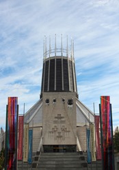
I’ve been working in Liverpool for a few months now, I take the Merseyrail train into Liverpool Central and then walk up the hill to ScraperWiki’s offices which are next door to the Liverpool Metropolitan Cathedral aka “Paddy’s Wigwam”.

Liverpool Metropolitan Cathedral

The cathedral was built in the 1960s, I rather like it. It looks to me like part of a set from a futuristic sci-fi film, maybe Gattacca or Equilibrium. Or some power collection or communication device, which in a way I suppose it is.

Liverpool Metropolitan Cathedral

To be honest the rest of my usual walk up the Brownlow Hill is coloured by a large, fugly carpark and a rather dodgy looking pub. However, these last few weeks the Merseyrail’s Liverpool Loop has been closed to re-lay track so I’ve walked across town from the James’ Street station, giving me the opportunity to admire some of Liverpool’s other architecture.

As an aside, it turns out that Merseyrail is the second oldest underground urban railway in the world, opening in 1886 and also originally running on steam power according to wikipedia, which seems to contradict Christian Wolmar in his book on the London Underground, which I recently reviewed. (Wolmar states the London Underground is the only one to have run on steam power.

Returning to architecture, I leave James’ Street station via the pedestrian exit on Water Street, there is a lift up onto James’ Street but I prefer the walk. As I come out there is a glimpse of the Royal Liver Building, on the waterfront.

Royal Liver Building

Just along the road is Liverpool Town Hall, for some reason it’s offset slightly from the centre of Castle Street which spoils the vista a little.

Liverpool Town HallDown at the other end of Castle Street we find the Queen Victoria Monument, she stands in Derby Square in front of the rather unattractive Queen Elizabeth II Law Courts.

Queen Victoria Monument

On the way I pass the former Adelphi Bank building, now a Cafe Nero. I like the exuberant decoration and the colour of the stone and domes.

Former Adelphi Bank


Raise your eyes from ground level and you see more decoration at the roof line of the buildings on Castle Street:

Buildings on Castle Street Once I’ve passed the Victoria Monument it’s a long straight walk down Lord Street then Church Street which has a mixture of buildings, many quite modern but some a bit older, often spoiled by the anachronistic shop fronts at street-level.

61 Lord Street

I quite like this one at 81-89 Lord Street but it’s seen better days, it used to look like this. It looks like it used to have a spectacular interior.

81-89 Lord Street


Further along, on Church Street, there is a large M&S in a fine building.

35 Church Street


35 Church Street


By now I’ve almost reached my normal route into work from Liverpool Central station, just around the corner on Renshaw Street is Grand Central Hall, which started life as a Methodist church.

Grand Central Hall

It’s a crazy looking building, the buddleia growing out of the roof make me think of one of J.G. Ballard’s novels.

Grand Central Hall

We’re on the final straight now, heading up Mount Pleasant towards the Metropolitan Cathedral. Looking back we can see the Radio City Tower, actually we can see the Radio City Tower from pretty much anywhere in Liverpool.

Radio City Tower

A little before we reach the Metropolitan Cathedral there is the YMCA on Mount Pleasant, another strange Victorian Gothic building.

YMCA Mount Pleasant

I struggled to get a reasonable photograph of this one, I was using my 28-135mm lens on a Canon 600D for this set of photos. This is a good walking around lens but for photos of buildings in dense city environments the 10-22mm lens is better for its ridiculously wide angle view – handy for taking pictures of all of a big building when you are standing next to it!

So maybe next week I’ll head out with the wide angle lens and apply some of the rectilinear correction I used on my Chester photographs.

pdftables – a Python library for getting tables out of PDF files

This post was first published at ScraperWiki.

One of the top searches bringing people to the ScraperWiki blog is “how do I scrape PDFs?” The answer typically being “with difficulty”, but things are getting better all the time.

PDF is a page description format, it has no knowledge of the logical structure of a document such as where titles are, or paragraphs, or whether it’s two column format or one column. It just knows where characters are on the page. The plot below shows how characters are laid out for a large table in a PDF file.

AlmondBoard7_LTChar

This makes extracting structured data from PDF a little challenging.

Don’t get me wrong, PDF is a useful format in the right place, if someone sends me a CV – I expect to get it in PDF because it’s a read only format. Send it in Microsoft Word format and the implication is that I can edit it – which makes no sense.

I’ve been parsing PDF files for a few years now, to start with using simple online PDF to text converters, then with pdftohtml which gave me better location data for text and now using the Python pdfminer library which extracts non-text elements and as well as bonding words into sentences and coherent blocks. This classification is shown in the plot below, the blue boxes show where pdfminer has joined characters together to make text boxes (which may be words or sentences). The red boxes show lines and rectangles (i.e. non-text elements).

AlmondBoard7

More widely at ScraperWiki we’ve been processing PDF since our inception with the tools I’ve described above and also the commercial, Abbyy software.

As well as processing text documents such as parliamentary proceedings, we’re also interested in tables of numbers. This is where the pdftables library comes in, we’re working towards making scrapers which are indifferent to the format in which a table is stored, receiving them via the OKFN messytables library which takes adapters to different file types. We’ve already added support to messytables for HTML, now its time for PDF support using our new, version-much-less-than-one pdftables library.

Amongst the alternatives to our own efforts are Mozilla’s Tabula, written in Ruby and requiring the user to draw around the target table, and Abbyy’s software which is commercial rather than open source.

pdftables can take a file handle and tell you which pages have tables on them, it can extract the contents of a specified page as a single table and by extension it can return all of the tables of a document (at the rate of one per page). It’s possible, for simple tables to do this with no parameters but for more difficult layouts it currently takes hints in the form of words found on the top and bottom rows of the table you are looking for. The tables are returned as a list of list of lists of strings, along with a diagnostic object which you can use to make plots. If you’re using the messytables library you just get back a tableset object.

It turns out the defining characteristic of a data scientist is that I plot things at the drop of a hat, I want to see the data I’m handling. And so it is with the development of the pdftables algorithms. The method used is inspired by image analysis algorithms, similar to the Hough transforms used in Tabula. A Hough transform will find arbitrarily oriented lines in an image but our problem is a little simpler – we’re interested in vertical and horizontal rows.

To find these vertical rows and columns we project the bounding boxes of the text on a page onto the horizontal axis ( to find the columns) and the vertical axis to find the rows. By projection we mean counting up the number of text elements along a given horizontal or vertical line. The row and column boundaries are marked by low values, gullies, in the plot of the projection. The rows and columns of the table form high mountains, you can see this clearly in the plot below. Here we are looking at the PDF page at the level of individual characters, the plots at the top and left show the projections. The black dots show where pdftables has placed the row and column boundaries.

AlmondBoard8_projection

pdftables is currently useful for supervised use but not so good if you want to just throw PDF files at it. You can find pdftables on Github and you can see the functionality we are still working on in the issue tracker. Top priorities are finding more than one table on a page and identifying multi-column text layouts to help with this process.

You’re invited to have a play and tell us what you think – [email protected]

Book review: The Subterranean Railway by Christian Wolmar

large-the-subterranean-railwayTo me the London underground is an almost magically teleportation system which brings order to the chaos of London. This is because I rarely visit London and know it only via Harry Beck’s circuit diagram map of the underground. To find out more about the teleporter, I have read The Subterranean Railway by Christian Wolmar.

London’s underground system was the first in the world, it predated any others by nearly 40 years. This had some drawbacks, for the first 30 years of its existence it ran exclusively using steam engines which are not good in an enclosed, underground environment. In fact travel in the early years of the Underground sounds really rather grim, despite its success.

The context for the foundation of the Underground was the burgeoning British rail network, it had started with one line between Manchester and Liverpool in 1830 by 1850 the country had a system spanning the country. The network did not penetrate to the heart of London, it had been stopped by a combination of landowner interests and expense. This exclusion was enshrined in the report of the 1846 Royal Commission on Metropolis Railway Termini. This left London with an ever-growing transport problem, now increased by the railway’s ability to get people to the perimeter of the city but no further.

The railways were the largest human endeavours since Roman times, as well as the engineering challenges there were significant financial challenges in raising capital and political challenges in getting approval. This despite the fact the the railway projectors were exempted from the restrictions on raising capital from groups of more than five people introduced after the South Seas Bubble.

The first underground line, the Metropolitan, opened in 1863 it ran from Paddington to Farringdon – it had been 20 years in the making, although construction only took 3 years. The tunnels were made by the cut-and-cover method, which works as described – a large trench is dug, the railway built in the bottom and then covered over. This meant the tunnels were relatively shallow, mainly followed the line of existing roads and involved immense disruption on the surface.

In 1868 the first section of the District line opened, this was always to be the Metropolitan’s poorer relative but would form part of the Circle line, finally completed in 1884 despite the animosity between James Staats Forbes and Edward Watkin – the heads of the respective companies at the time. It’s worth noting that it wasn’t until 1908 that the first London Underground maps were published; in its early days the underground “system” was the work of disparate private companies who were frequently at loggerheads and certainly not focussed on cooperating to the benefit of their passengers.

The underground railways rarely provided the returns their investors were looking for but they had an enormous social impact, for the first time poorer workers in the city could live out of town in relatively cheap areas and commute in, the railway companies positively encouraged this. The Metropolitan also invested in property in what are now the suburbs of London, areas such as Golders Green were open fields before the underground came. This also reflects the expansion of the underground into the surrounding country.

The first deep line, the City and South London was opened in 1890, it was also the first electric underground line. The deep lines were tunnelled beneath the city using the tunnelling shield developed by Marc Brunel, earlier in the 19th century. Following the first electrification the District and Metropolitan lines eventually electrified their lines, although it took some time (and a lot of money). The finance for the District line came via the American Charles Tyson Yerkes, who would generously be described as a colourful character, engaging in financial engineering which we likely imagine is a recent invention.

Following the First World War the underground was tending towards a private monopoly, government was looking to invest to make work and ultimately the underground was nationalised, at arms length, to form London Transport in 1933, led by the same men (Lord Ashfield and Frank Pick) who had run the private monopoly.

The London underground reached its zenith in the years leading up to the Second World War, gaining its identity (roundel, font and iconic map) and forming a coherent, widespread network. After the war it was starved of funds, declining – overtaken by the private car. Further lines were added such as the Victoria and Jubilee lines but activity was much reduced from the early years.

More recently it has seen something of a revival with the ill-fated Public-Private Partnership running into the ground, but not before huge amounts of money had been spent, substantially on improvements. As I write, the tunnelling machines are building Crossrail.

I felt the book could have done with a construction timeline, something like this on wikipedia (link), early on there seems to be a barrage of new line openings, sometimes not in strictly chronological order and to someone like me, unfamiliar with London it is all a bit puzzling. Despite this The Subterranean Railway is an enjoyable read.